Visualizing sort algorithms with ggplot2

Have you read Visualizing Algorithms by Mike Bostock? It’s a pure gold post. In that post Mike show a static representation of a sort algorithm and obvious it will fun to replicate that image with ggplot2 so here we go.

We need some sorts algorithms. In this link you can see some algorithms.

We start with Insertion sort:

library(dplyr)
library(tidyr)
library(ggplot2)
library(viridis)

theme_set(theme_void())

insertion_sort_steps <- function(x  = sample(1:15)){
  
  msteps <- matrix(data = x, ncol = length(x))
  
  for (i in 2:length(x)) {
    
    j <- i
    
    while ((j > 1) && (x[j] < x[j - 1])) {
      
      temp <- x[j]
      x[j] <- x[j - 1]
      x[j - 1] <- temp
      j <- j - 1
      
      msteps <- rbind(msteps, as.vector(x))
      
    }
  }
  
  msteps
  
}

Now to test it and see what the function do:

set.seed(12345)

x <- sample(seq(4))

x

[1] 2 3 4 1

msteps <- insertion_sort_steps(x)

as.data.frame(msteps)

  V1 V2 V3 V4
1  2  3  4  1
2  2  3  1  4
3  2  1  3  4
4  1  2  3  4

Every row is a step in sort the algorithm (a partial sort). This matrix is a hard to plot so we need a nicer structure. We can transform the matrix to a data_frame with the information of every position of every element in each step.

sort_matix_to_df <- function(msteps){
  
  df <- as.data.frame(msteps, row.names = NULL)
  
  names(df) <- seq(ncol(msteps))
  
  df_steps <- df %>%
    tibble::as_tibble() %>% 
    mutate(step = seq(nrow(.))) %>% 
    gather(position, element, -step) %>%
    arrange(step)
  
  df_steps
  
}

And we apply this function to the previous steps matrix.

df_steps <- sort_matix_to_df(msteps)

head(df_steps, 10)

# A tibble: 10 × 3
    step position element
   <int> <chr>      <int>
 1     1 1              2
 2     1 2              3
 3     1 3              4
 4     1 4              1
 5     2 1              2
 6     2 2              3
 7     2 3              1
 8     2 4              4
 9     3 1              2
10     3 2              1

The next step will be plot the data frame.

plot_sort <- function(df_steps, size = 5, color.low = "#D1F0E1", color.high = "#524BB4"){
  
  ggplot(df_steps,
         aes(step, position, group = element, color = element, label = element)) +  
    geom_path(size = size, alpha = 1, lineend = "round") +
    scale_colour_gradient(low = color.low, high = color.high) +
    coord_flip() + 
    scale_x_reverse() + 
    theme(legend.position = "none")
  
}

Now compare this:

as.data.frame(msteps)

  V1 V2 V3 V4
1  2  3  4  1
2  2  3  1  4
3  2  1  3  4
4  1  2  3  4

With:

plot_sort(df_steps, size = 6) + 
  geom_text(color = "white", size = 4)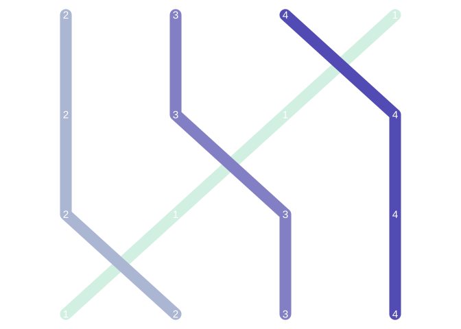

It works, so we can now scroll!

sample(seq(50)) %>% 
  insertion_sort_steps() %>% 
  sort_matix_to_df() %>% 
  plot_sort(size = 2.0)

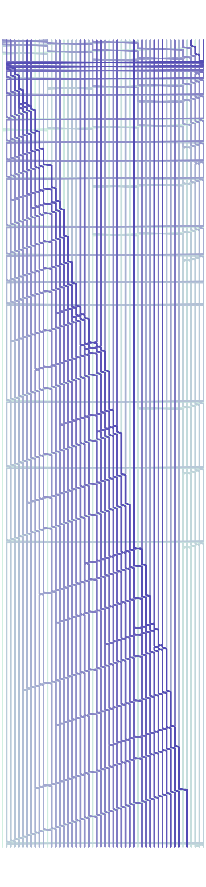
Now try with other sort algorithms:

Bubble sort:

bubble_sort_steps <- function(x = sample(1:15)){
  
  msteps <- matrix(data = x, ncol = length(x))
  
  for (i in 1:(length(x) - 1)) {
    
    for (j in 1:(length(x) - 1)) {
      
      if (x[j] > x[j + 1]) {
        temp <- x[j]
        x[j] <- x[j + 1]
        x[j + 1] <- temp
      }
      
      msteps <- rbind(msteps, as.vector(x))
      
    }
  }
  
  msteps
  
}

Selection sort:

selection_sort_steps <- function(x = sample(1:15)){
  
  msteps <- matrix(data = x, ncol = length(x))
  
  for (i in 1:(length(x) - 1)) {
    
    smallsub <- i
    
    for (j in (i + 1):(length(x) - 0)) { # Is not '- 1' like website
      
      if (x[j] < x[smallsub]) {
        smallsub <- j
      }
    }
    
    temp <- x[i]
    x[i] <- x[smallsub]
    x[smallsub] <- temp
    
    msteps <- rbind(msteps, as.vector(x))
    
  }
  
  msteps
  
}

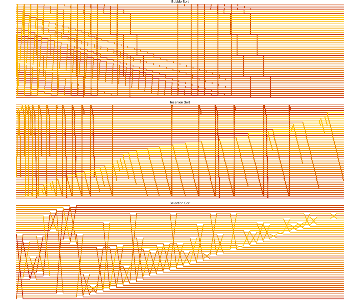
Now test with a longer vector:

n <- 50
x <- sample(seq(n))

big_df <- rbind(
  x %>% selection_sort_steps() %>% sort_matix_to_df() %>% mutate(sort = "Selection Sort"),  
  x %>% insertion_sort_steps() %>% sort_matix_to_df() %>% mutate(sort = "Insertion Sort"),
  x %>% bubble_sort_steps() %>% sort_matix_to_df() %>% mutate(sort = "Bubble Sort")
)

head(big_df)

# A tibble: 6 × 4
   step position element sort          
  <int> <chr>      <int> <chr>         
1     1 1             10 Selection Sort
2     1 2             43 Selection Sort
3     1 3             27 Selection Sort
4     1 4             34 Selection Sort
5     1 5             44 Selection Sort
6     1 6             35 Selection Sort

big_df %>%
  group_by(sort) %>% 
  summarise(steps = n())

# A tibble: 3 × 2
  sort            steps
  <chr>           <int>
1 Bubble Sort    120100
2 Insertion Sort  32100
3 Selection Sort   2500

ggplot(
  big_df,
  aes(step, position, group = element, color = element, label = element)
  ) +  
  geom_path(size = 0.8, alpha = 1, lineend = "round") +
  scale_colour_gradient(low = "#c21500", high = "#ffc500") + # http://uigradients.com/#Kyoto
  facet_wrap(~sort, scales = "free_x", ncol = 1) +
  theme(
    legend.position = "none",
    strip.background = element_rect(fill = "transparent", linetype = 0),
    strip.text = element_text(size = 8)
    )

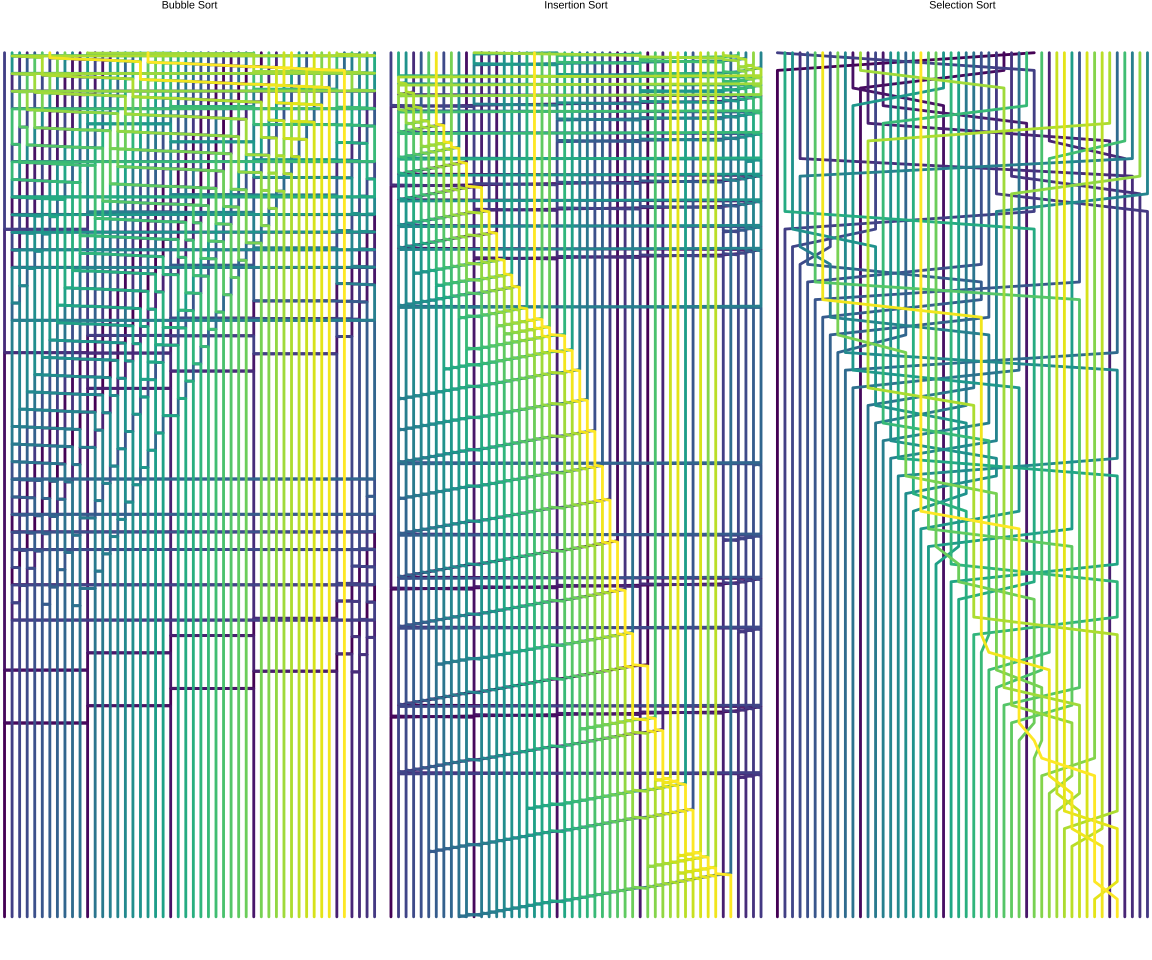
Or we can plot vertically using the viridis palette from the viridis package :

ggplot(
  big_df,
  aes(position, step, group = element, color = element, label = element)
  ) +  
  geom_path(size = 1, alpha = 1, lineend = "round") +
  scale_colour_gradientn(colours = viridis_pal()(n)) +
  facet_wrap(~sort, scales = "free_y", nrow = 1) +
  scale_y_reverse() +
  theme(
    legend.position = "none",
    strip.background = element_rect(fill = "transparent", linetype = 0),
    strip.text = element_text(size = 8)
    )

And that’s it. If you write/implement another sort algorithm in this way let me know to view it ;).

References:

http://bost.ocks.org/mike/algorithms/
http://faculty.cs.niu.edu/~hutchins/csci230/sorting.htm
http://corte.si/posts/code/visualisingsorting/
http://uigradients.com/#Kyoto
http://algs4.cs.princeton.edu/21elementary/