Nürburgring, One Geom at a Time

Draw racetracks, roads and trails with OpenStreetMap and ggplot2.
R
maps
ggplot2
OpenStreetMap
Author

Joshua Kunst

Published

September 10, 2026

OpenStreetMap gives us enough detail to draw the Nürburgring without a basemap. In this post we build the map progressively: first the surrounding road network, then line-width hierarchy, waterways and the racetrack itself, finishing with a few named Nordschleife sections and the Sprintstrecke.

The palette follows the place rather than a generic map style. Forest green nods to the Nordschleife’s Green Hell nickname, while cool asphalt greys keep the surrounding roads quiet.

A stylised map of Nürburgring with the racetrack highlighted against the surrounding road network.

Map area

Set the screen resolution, map width and palette here. Height follows the screen ratio. Reduce width_km to zoom in; extra_area_pct adds space around the shared map view. The download uses the coordinates below; the visible maps are centred on the racetrack bounds, with optional east/north shifts for fine-tuning.

# Map palette: forest green for the circuit and cool asphalt greys for the canvas.
forest_green <- "#47714D"
asphalt_light <- "#E3E8EB"
asphalt_dark <- "#30373D"

# 1440p in landscape orientation.
screen_width_px <- 2560
screen_height_px <- 1440
# Sets text and stroke scale at the requested pixel dimensions.
export_dpi <- 160

# Download centre: longitude in decimal degrees, east of Greenwich.
centre_lon <- 6.95
# Download centre: latitude in decimal degrees, north of the equator.
centre_lat <- 50.35
# Lower this to show less space around the circuit.
width_km <- 14
# Extra area around the shared map view.
extra_area_pct <- 15
# Trim the visible frame without changing the cached download area.
visible_crop_pct <- 14
# Optional offset from the racetrack centre: positive east moves the track left.
map_shift_east_km <- 0
# Positive north moves the track down; zero keeps it vertically centred.
map_shift_north_km <- 0

stopifnot(screen_width_px > 0, screen_height_px > 0, export_dpi > 0,
          width_km > 0, extra_area_pct >= 0,
          visible_crop_pct >= 0, visible_crop_pct < 100)

# Match the geographic frame to the screen without stretching the roads.
screen_ratio <- screen_width_px / screen_height_px
height_km <- width_km / screen_ratio

# Keep the same proportions for the maps in the post and the wallpaper exports.
knitr::opts_chunk$set(fig.asp = 1 / screen_ratio)

# Show the projected frame areas before making any download request.
c(detail_km2 = width_km * height_km,
  surroundings_km2 = width_km * height_km * (1 + extra_area_pct / 100))
      detail_km2 surroundings_km2 
        110.2500         126.7875 

Build the download frame in metres using the local UTM projection.

# EPSG:4326 identifies longitude/latitude coordinates in WGS84.
centre <- sf::st_sfc(sf::st_point(c(centre_lon, centre_lat)), crs = 4326) |>
  # ETRS89 / UTM zone 32N uses metres in this region.
  sf::st_transform(25832) |>
  # Extract the projected x and y coordinates.
  sf::st_coordinates()

# Use a plain vector for the frame calculations.
centre <- as.numeric(centre)

make_frame <- function(width_m, height_m, frame_centre = centre) {
  # Half the width and height on each side keep the rectangle centred.
  sf::st_bbox(c(
    xmin = frame_centre[1] - width_m / 2,
    ymin = frame_centre[2] - height_m / 2,
    xmax = frame_centre[1] + width_m / 2,
    ymax = frame_centre[2] + height_m / 2
  ), crs = sf::st_crs(25832)) |>
    # Turn the bounds into a polygon for clipping and plotting.
    sf::st_as_sfc()
}

# Convert kilometres to the projection's metre units.
width_m <- width_km * 1000
height_m <- height_km * 1000

# Area = width × height: scale both sides by the square root of the area multiplier.
margin_scale <- sqrt(1 + extra_area_pct / 100)

download_frame <- make_frame(
  width_m * margin_scale,
  height_m * margin_scale
)

Data

Download once per area and save an RDS. The same settings reuse the file; changing them creates a separate cache.

# Include every area setting so a different frame cannot reuse the wrong data.
area_id <- paste(centre_lon, centre_lat, width_km, height_km, extra_area_pct, sep = "_")

osm_file <- file.path("data", paste0("osm-", area_id, ".rds"))

if (!file.exists(osm_file)) {
  # Overpass needs longitude/latitude bounds; their envelope is slightly larger.
  bbox_wgs84 <- download_frame |> sf::st_transform(4326) |> sf::st_bbox()
  # Ways contain the road and river geometry; timeout is a server time limit in seconds.
  query <- osmdata::opq(bbox = bbox_wgs84, osm_types = "way", timeout = 180) |>
    # The plural function combines filters with OR: highways OR rivers/streams.
    # Match these waterway values exactly.
    osmdata::add_osm_features(features = c(
      '"highway"', '"waterway"~"^(river|stream)$"'
    ))

  message("Downloading and converting roads and rivers...")
  # Convert the response to sf objects and show progress messages.
  osm <- osmdata::osmdata_sf(query, quiet = FALSE)

  # Keep only the line layer used below.
  osm <- list(osm_lines = osm$osm_lines)

  message("Saving data...")
  dir.create(dirname(osm_file), recursive = TRUE, showWarnings = FALSE)
  saveRDS(osm, osm_file)
}

osm <- readRDS(osm_file)

# Tighten the visible frame without changing the cached download area.
visible_scale <- 1 - visible_crop_pct / 100
visible_width_m <- width_m * visible_scale
visible_height_m <- height_m * visible_scale

The query uses osmdata. Separate the roads and waterways into layers.

library(dplyr)

roads <- osm$osm_lines |>
  # The highway tag includes paths and racetracks.
  filter(!is.na(highway)) |>
  # Keep useful tags; sf retains the geometry.
  select(osm_id, name, highway) |>
  sf::st_transform(25832)

waterways <- osm$osm_lines |>
  filter(waterway %in% c("river", "stream")) |>
  sf::st_transform(25832)

# Measure the racetracks before clipping so the crop cannot bias their centre.
circuit_bbox <- roads |>
  filter(highway == "raceway") |>
  sf::st_bbox()

if (!all(is.finite(circuit_bbox))) {
  stop("No racetrack geometry found in the downloaded area.")
}

# Midpoints of the bounds give equal space on opposite sides of the racetracks.
circuit_centre <- c(
  (circuit_bbox[["xmin"]] + circuit_bbox[["xmax"]]) / 2,
  (circuit_bbox[["ymin"]] + circuit_bbox[["ymax"]]) / 2
)

# Convert the optional offsets from kilometres to metres.
map_centre <- circuit_centre + c(map_shift_east_km, map_shift_north_km) * 1000

map_frame <- make_frame(
  visible_width_m * margin_scale,
  visible_height_m * margin_scale,
  map_centre
)

# Reuse these bounds across every map in the post.
map_bbox <- sf::st_bbox(map_frame)

# Clip lines to the frame itself: Overpass may return ways that extend outside it.
roads_surroundings <- sf::st_intersection(roads, map_frame)
water_map <- sf::st_crop(waterways, map_bbox)

A quick look at the selected road fields keeps the following steps grounded in the data actually returned by OpenStreetMap.

roads |>
  sf::st_drop_geometry() |>
  glimpse()
Rows: 4,911
Columns: 3
$ osm_id  <chr> "10310943", "22723643", "26471548", "26471724", "26471730", "2…
$ name    <chr> NA, NA, NA, NA, "Kapellenstraße", NA, "Gartenstraße", "Herschb…
$ highway <chr> "secondary", "service", "tertiary", "tertiary", "residential",…

One line weight

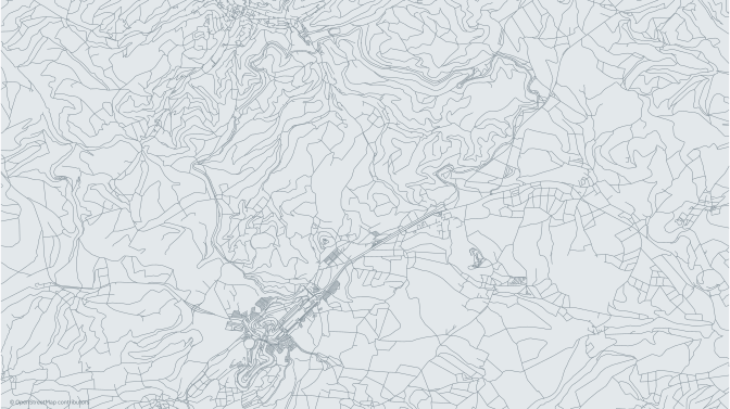
Start with every road drawn alike. Apply coord_sf() after the spatial layers to keep the explicit limits and expand = FALSE, avoiding an empty border around the clipped roads. A small credit sits inside the map; no scale bar, caption strip or outer margin is added to the wallpaper.

library(ggplot2)

# Reuse the blog's shared typography.
map_font <- theme_get()$text$family

# Matching panel and canvas backgrounds keep the wallpaper filled to its edges.
map_theme <- theme_void(base_family = map_font) +
  theme(
    panel.background = element_rect(fill = asphalt_light, colour = NA),
    plot.background = element_rect(fill = asphalt_light, colour = NA),
    plot.margin = margin(0, 0, 0, 0)
  )

# Put the credit inside either frame, without a text box or an external caption.
map_credit <- function(bounds = map_bbox, colour = "#62717A") {
  annotate(
    "text",
    # Inset the text 1.2% from the left and bottom edges of the projected frame.
    x = bounds[["xmin"]] + 0.012 * (bounds[["xmax"]] - bounds[["xmin"]]),
    y = bounds[["ymin"]] + 0.012 * (bounds[["ymax"]] - bounds[["ymin"]]),
    label = "© OpenStreetMap contributors",
    family = map_font,
    size = 1.4,
    colour = colour,
    hjust = 0,
    vjust = 0
  )
}

# Fixed limits let us compare styles without changing the close view.
map_coords <- coord_sf(
  crs = 25832,
  xlim = map_bbox[c("xmin", "xmax")],
  ylim = map_bbox[c("ymin", "ymax")],
  # Add no coordinate padding or latitude/longitude graticule.
  expand = FALSE,
  datum = NA
)

# Keep the canvas free of captions; add the credit after the road layers.
detail_canvas <- ggplot() +
  map_theme

uniform_map <- detail_canvas +
  geom_sf(
    data = roads_surroundings,
    colour = "#77858E",
    linewidth = 0.15
  ) +
  map_credit() +
  map_coords

uniform_map

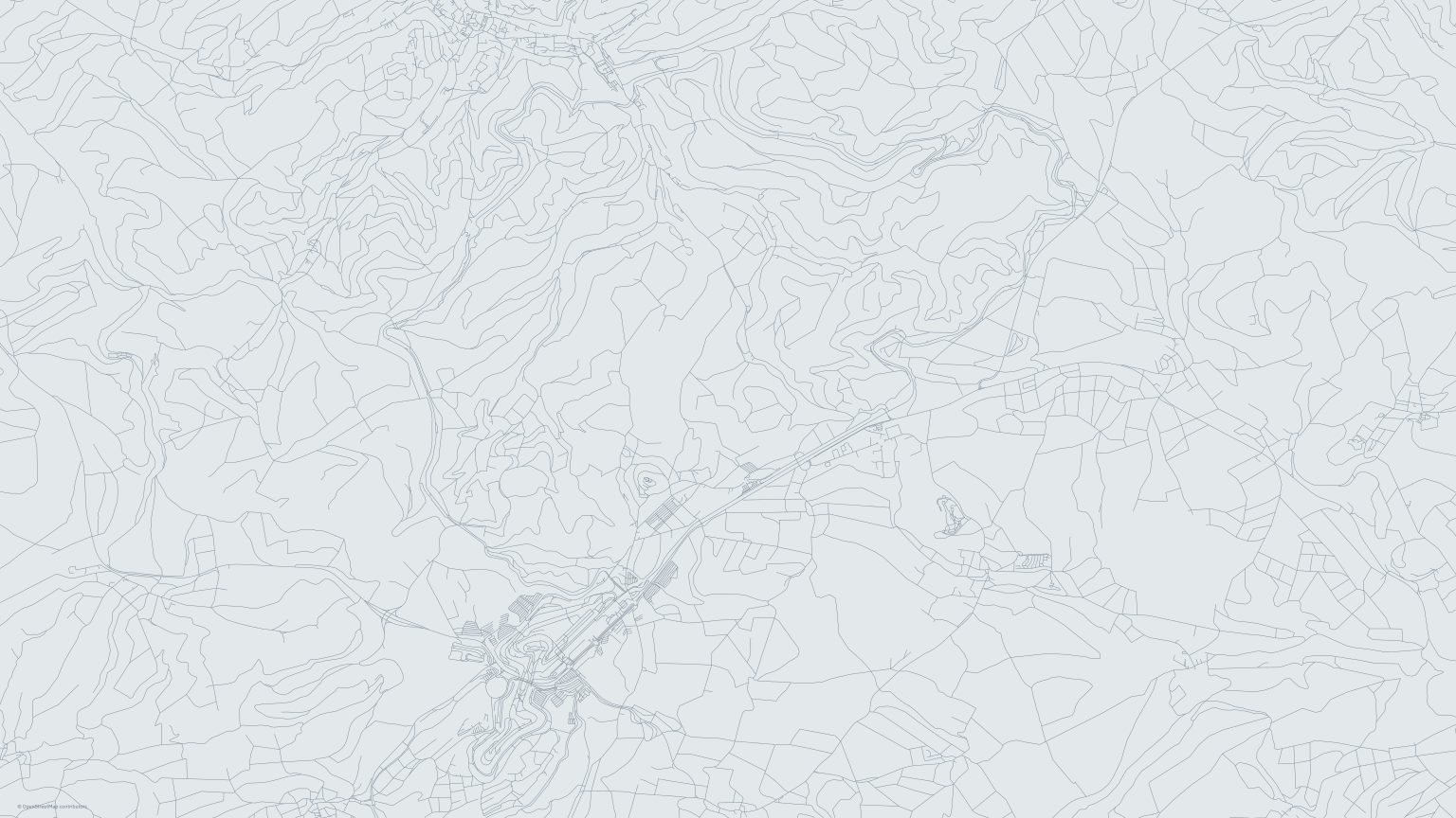
The road network around Nürburgring, drawn in thin grey lines on a light grey background.

Every road uses the same colour and line width.

Line widths

Use highway to set a visual hierarchy, including raceway for racetracks. The widths are design choices, rather than physical road measurements. Before defining broader visual groups, inspect which highway tags are present inside the shared map frame. Because the geometries use EPSG:25832, their lengths can also be summed directly in kilometres.

roads_surroundings |>
  mutate(length_km = as.numeric(sf::st_length(geometry)) / 1000) |>
  sf::st_drop_geometry() |>
  summarise(
    ways = n_distinct(osm_id),
    length_km = round(sum(length_km), 1),
    .by = highway
  ) |>
  arrange(desc(length_km))
          highway ways length_km
1           track 1459     591.2
2         service  953      98.6
3     residential  387      59.6
4            path  197      46.3
5        tertiary  132      44.2
6         primary  156      37.3
7         raceway   98      29.3
8         footway  154      15.8
9       secondary   53      15.0
10   unclassified   45       8.2
11   primary_link   15       1.6
12          steps   53       0.9
13  living_street    1       0.3
14 secondary_link    4       0.2
15     pedestrian    1       0.2
16  tertiary_link    2       0.1

For comparison, the official Nürburgring record definitions list the Nordschleife at 20.832 km and the Grand Prix Track at 5.148 km. The OSM raceway total is a geometry check over all raceway-tagged ways in the frame, not an official circuit length.

The name tag shows how that total is split across the raceway ways. Missing names stay visible as Unnamed rather than being dropped. The full list is kept collapsed because OSM names many individual track sections, not just whole circuits.

Code
raceways <- roads_surroundings |>
  filter(highway == "raceway") |>
  mutate(
    raceway_name = coalesce(name, "Unnamed"),
    length_km = as.numeric(sf::st_length(geometry)) / 1000
  )

raceway_summary <- raceways |>
  sf::st_drop_geometry() |>
  summarise(
    ways = n_distinct(osm_id),
    length_km = round(sum(length_km), 2),
    .by = raceway_name
  ) |>
  arrange(desc(length_km))

cat("<details>\n")
Code
cat("<summary>Show all ", nrow(raceway_summary), " raceway names</summary>\n\n", sep = "")
Show all 60 raceway names
Code
cat('<div style="max-height: 22rem; overflow-y: auto;">\n')
Code
cat(knitr::kable(raceway_summary, format = "html"))
raceway_name ways length_km
Nürburgring Sprintstrecke 9 3.62
Unnamed 18 1.60
Boxengasse 3 1.19
Hohe Acht 1 1.12
Antoniusbuche 1 0.90
Fuchsröhre 1 0.86
Kesselchen 1 0.79
Schwedenkreuz 1 0.76
Pflanzgarten 1 0.76
Döttinger Höhe 1 0.75
Metzgesfeld 1 0.71
Flugplatz 1 0.70
Galgenkopf 1 0.69
Senkenlinks 1 0.67
Hatzenbach 1 0.59
Boxengasse an T13 7 0.53
Hocheichen 1 0.53
Steilstrecke 1 0.53
Kallenhard 1 0.52
Adenauer Forst 1 0.50
Brünnchen 1 0.49
Schwalbenschwanz 1 0.49
Breidscheid 3 0.48
Hatzenbogen 1 0.47
Stefan-Bellof-S 1 0.43
Eschbach 1 0.42
Exmühle 1 0.40
Wehrseifen 1 0.40
Bergwerk 1 0.40
Hohenrain 1 0.39
Rallycross circuit turn 8a 1 0.39
Aremberg 1 0.38
Mutkurve 1 0.38
Mini-Karussell 1 0.38
Lauda-Links 1 0.36
Klostertal 1 0.35
Quiddelbacher Höhe 1 0.34
Dreifach-Rechts 1 0.34
Wippermann 1 0.32
Tiergarten 1 0.29
Rallycross circuit 4 0.29
Sprunghügel 1 0.26
Michael-Schumacher-S 1 0.24
Goodyear-Kehre 1 0.23
T13 1 0.20
Spiegelkurve 1 0.19
Eiskurve 1 0.19
Müllenbachschleife 1 0.18
Hedwigshöhe 1 0.16
Karussell 1 0.15
Anbindung zum GP Kurs 1 0.14
Variante 24h-Rennen 1 0.14
Ford-Kurve 1 0.13
NGK-Schikane 1 0.12
Anbindung zur Sprintstrecke 1 0.12
Sabine-Schmitz-Kurve 1 0.11
Anbindung zur Nordschleife 1 0.10
Anbindung zur Müllenbachschleife 1 0.07
Rallycross Circuit 1 0.04
Nürburgring Nordschleife 1 0.03
Code
cat("\n</div>\n\n</details>\n")

Keep every road group, but give minor paths thinner, quieter lines and the circuit a stronger stroke.

# Combine related OSM tags so each road group can share one style.
roads_surroundings <- roads_surroundings |>
  mutate(road_group = case_match(
    highway,
    "raceway" ~ "Racetracks",
    c("motorway", "motorway_link") ~ "Motorways",
    c("trunk", "trunk_link", "primary", "primary_link") ~
      "Main roads",
    c("secondary", "secondary_link", "tertiary", "tertiary_link") ~
      "Regional roads",
    c("residential", "living_street", "unclassified") ~
      "Local roads",
    "service" ~ "Service roads",
    "track" ~ "Farm and forest tracks",
    c("path", "footway", "cycleway", "bridleway", "steps", "pedestrian") ~
      "Non-motorised paths",
    .default = "Other"
  ))

# The table order also sets the drawing order, from quietest to strongest.
road_style <- tibble::tribble(
  ~road_group,                ~line_width, ~line_colour, ~dark_colour,
  "Other",                         0.06, "#D3DADE",    "#3C4449",
  "Non-motorised paths",           0.06, "#CCD5DA",    "#404A50",
  "Farm and forest tracks",        0.08, "#C0CBD1",    "#48545B",
  "Service roads",                 0.10, "#B6C2C9",    "#515F67",
  "Local roads",                   0.14, "#A4B2BA",    "#60717A",
  "Regional roads",                0.23, "#8B9DA7",    "#788E9A",
  "Main roads",                    0.30, "#738A96",    "#90A6B1",
  "Motorways",                     0.38, "#58727E",    "#A6BAC4",
  "Racetracks",                    1.10, forest_green,  "#E0EFD9"
)

roads_surroundings <- roads_surroundings |>
  # Attach widths and colours to each road.
  left_join(road_style, by = "road_group") |>
  # Preserve the table order when drawing the layers.
  mutate(road_group = factor(road_group, levels = road_style$road_group)) |>
  arrange(road_group)

Keep the colour constant to see what line width changes.

width_map <- detail_canvas +
  geom_sf(
    data = roads_surroundings,
    aes(linewidth = line_width),
    colour = "#77858E",
    lineend = "round"
  ) +
  # Use the table's widths directly, without rescaling.
  scale_linewidth_identity() +
  map_credit() +
  map_coords

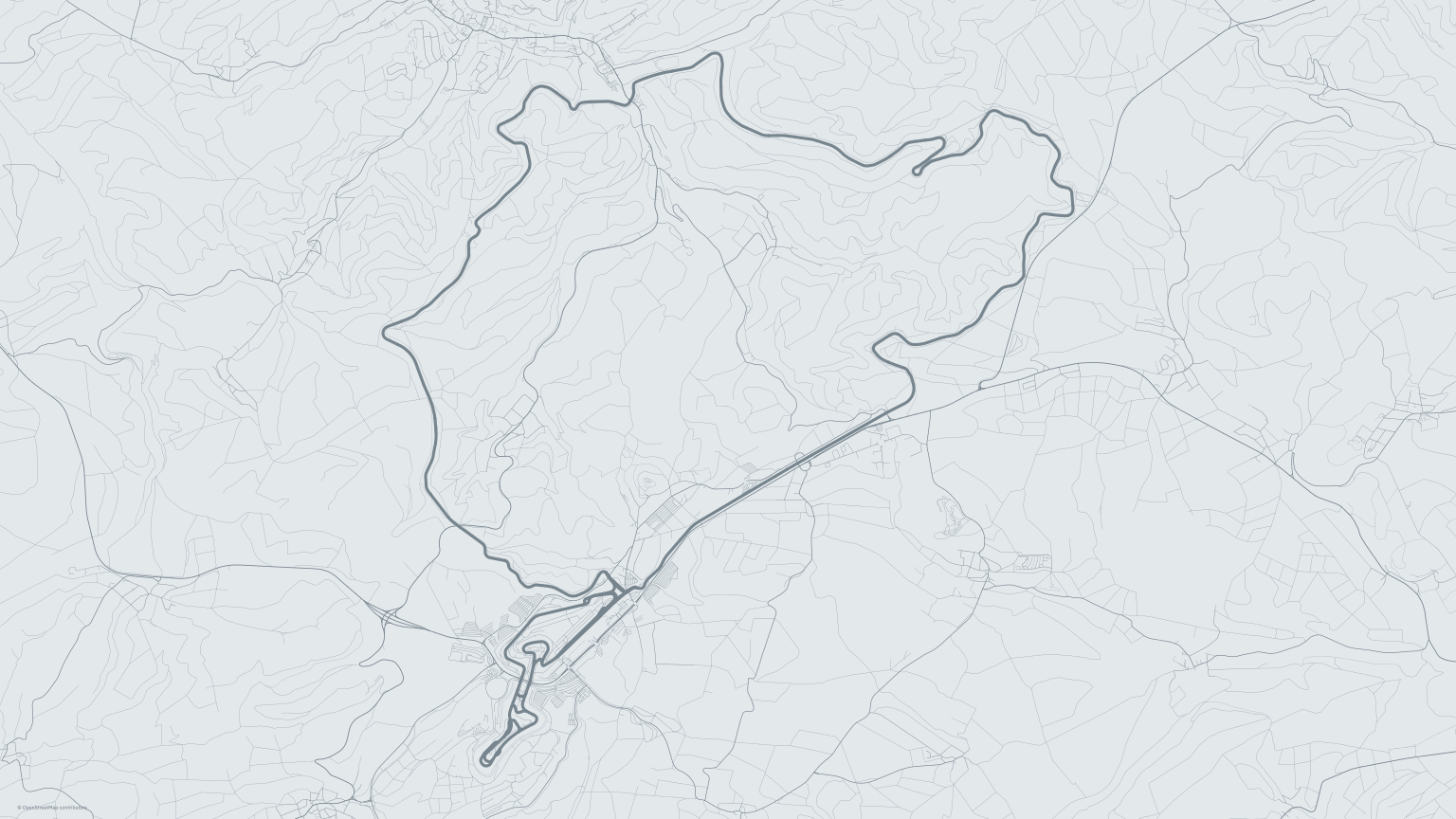
width_map

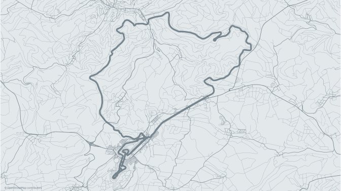
The same grey road network, with thicker strokes for racetracks and major roads.

Line width separates the main roads from minor paths.

Surroundings and the circuit

Add colour and rivers first, keeping the racetrack out of the surrounding road layer. Faint blue-grey lines are minor roads and paths, including forest tracks; pale blue lines are waterways.

water_colour <- "#B7C9D1"

roads_context <- roads_surroundings |>
  filter(road_group != "Racetracks")

surroundings_map <- detail_canvas +
  # Water goes below roads so the road hierarchy stays legible at crossings.
  geom_sf(
    data = water_map,
    colour = water_colour,
    linewidth = 0.10
  ) +
  geom_sf(
    data = roads_context,
    aes(colour = line_colour, linewidth = line_width),
    lineend = "round"
  ) +
  scale_colour_identity() +
  scale_linewidth_identity() +
  map_credit() +
  map_coords

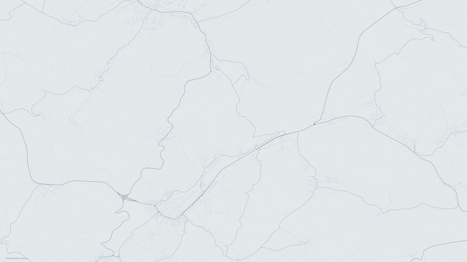
surroundings_map

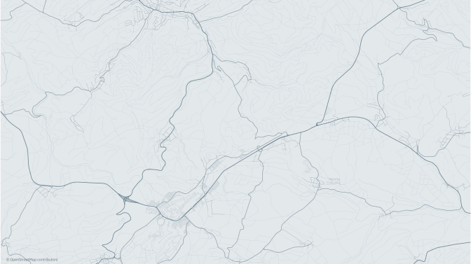
A map of the roads around Nürburgring, with blue-grey road hierarchy and pale waterways but no highlighted racetrack.

The surrounding road network before the racetrack is added.

With the context in place, the Nürburgring is one more geometry: add the ways tagged as raceway on top of the same map.

detail_map <- surroundings_map +
  geom_sf(
    data = raceways,
    colour = forest_green,
    linewidth = 1.10,
    lineend = "round",
    inherit.aes = FALSE
  )

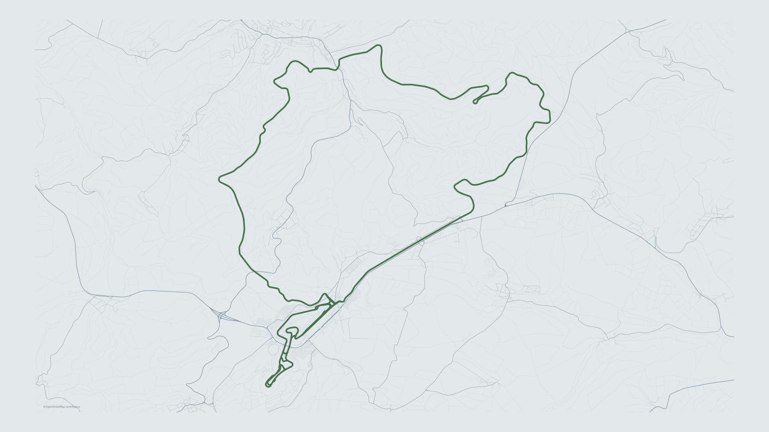
detail_map

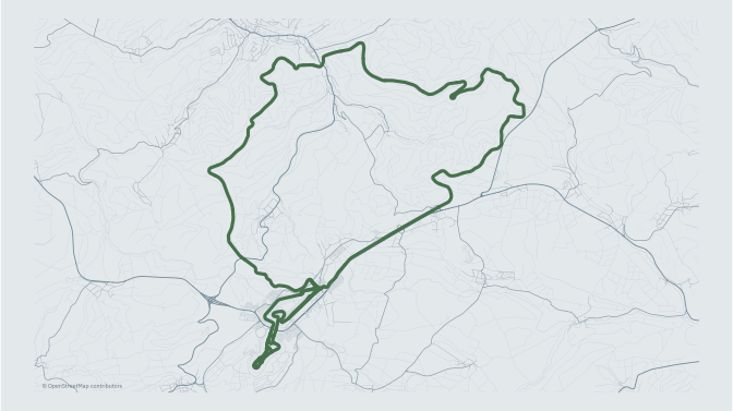
Nürburgring in forest green, highlighted over a blue-grey surrounding road network on a pale asphalt background.

The racetrack added as one final geometry over the surrounding roads.

A darker version

The light version uses a cool asphalt grey. Blue-charcoal and lighter roads give the same map a darker treatment. The preview uses muted forest green (#47714D).

Code
# Reuse the exact frame and geometries; only the palette changes.
dark_map <- detail_canvas +
  geom_sf(
    data = water_map,
    colour = "#43545E",
    linewidth = 0.10
  ) +
  geom_sf(
    data = roads_surroundings,
    aes(colour = dark_colour, linewidth = line_width),
    lineend = "round"
  ) +
  scale_colour_identity() +
  scale_linewidth_identity() +
  # Match both backgrounds and lighten the overlaid credit for this palette.
  theme(
    panel.background = element_rect(fill = asphalt_dark, colour = NA),
    plot.background = element_rect(fill = asphalt_dark, colour = NA)
  ) +
  map_credit(colour = "#A6B6C0") +
  map_coords

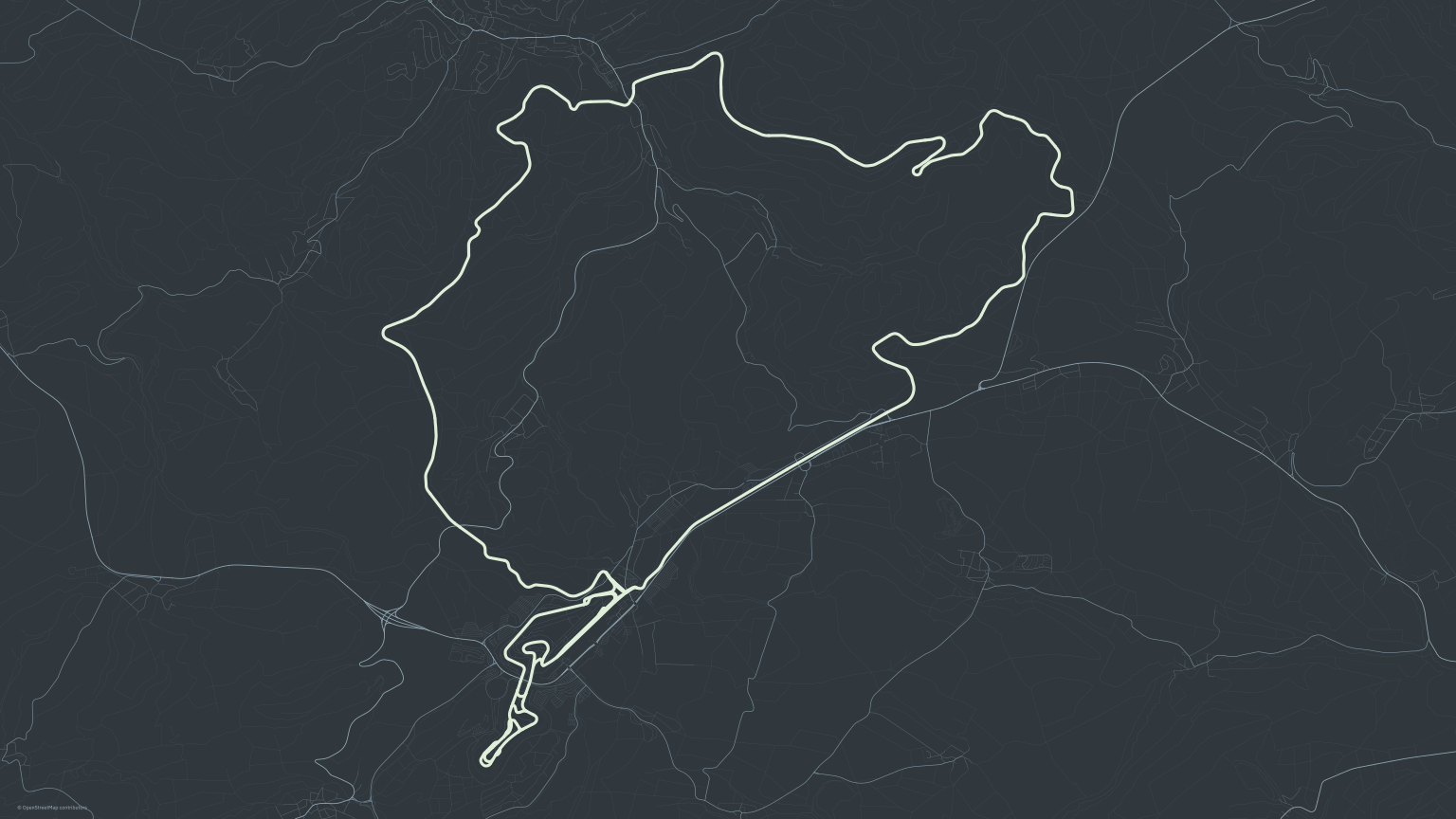
dark_map

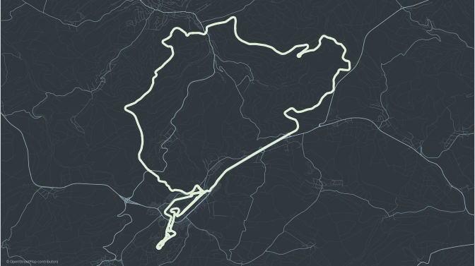
Nürburgring in pale green against blue-charcoal, with muted blue-grey roads and streams.

The same roads and frame, with colours adjusted for a charcoal background.

Circuit details

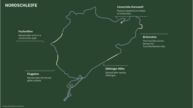
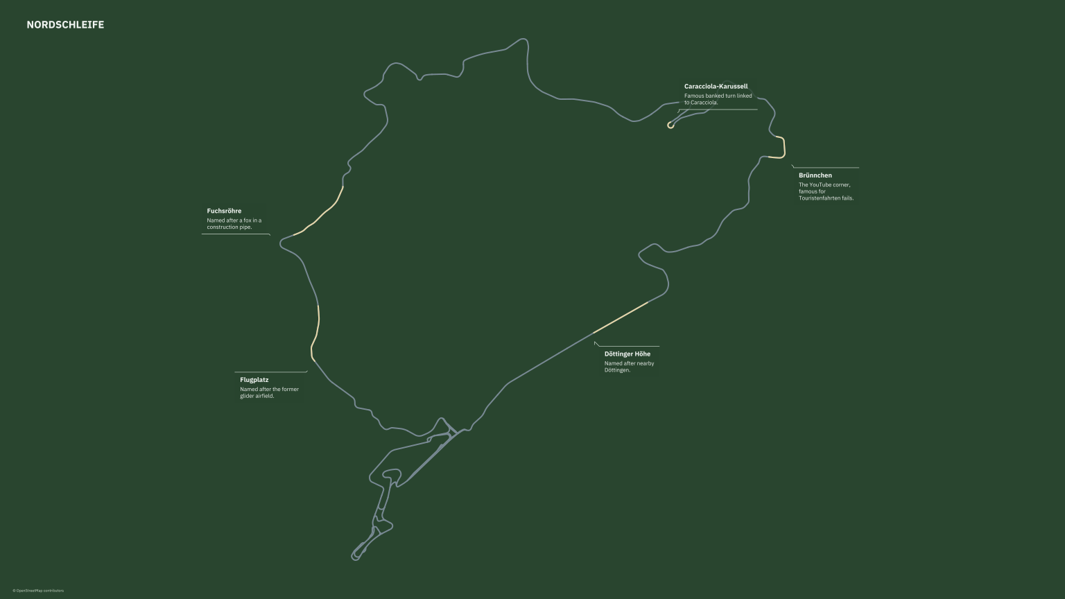
OpenStreetMap stores the Nordschleife as individually named raceway ways. Rather than marking each section as a point, keep the actual line geometry and let ggforce::geom_mark_hull() anchor each annotation to the full highlighted section. For this annotated view, remove the surrounding roads and waterways so the raceway geometry stays in focus. The short annotations below paraphrase the official Nürburgring Nordschleife guide.

section_names <- c(
  "Fuchsröhre",
  "Flugplatz",
  "Döttinger Höhe",
  "Karussell",
  "Brünnchen"
)

featured_raceways <- raceways |>
  filter(raceway_name %in% section_names)

section_descriptions <- tibble::tribble(
  ~section,           ~description,
  "Fuchsröhre",       "Named after a fox in a construction pipe.",
  "Flugplatz",        "Named after the former glider airfield.",
  "Döttinger Höhe",   "Named after nearby Döttingen.",
  "Karussell",        "Famous banked turn linked to Caracciola.",
  "Brünnchen",        "The YouTube corner, famous for Touristenfahrten fails."
)

track_sections <- featured_raceways |>
  mutate(section = raceway_name) |>
  group_by(section) |>
  summarise() |>
  mutate(section_label = if_else(section == "Karussell", "Caracciola-Karussell", section)) |>
  left_join(section_descriptions, by = "section") |>
  mutate(label = section_label)

# Densify the same section lines so the annotation stays tied to the full segment.
section_hull_points <- track_sections |>
  sf::st_segmentize(dfMaxLength = 25) |>
  sf::st_cast("POINT", warn = FALSE)

section_xy <- sf::st_coordinates(section_hull_points)
section_hull_points <- section_hull_points |>
  mutate(
    x = section_xy[, 1],
    y = section_xy[, 2]
  )

# Fix annotation anchors around the outside of the track instead of letting them float.
section_label_positions <- tibble::tribble(
  ~section,           ~x_frac, ~y_frac,
  "Fuchsröhre",          0.14,    0.72,
  "Flugplatz",           0.20,    0.28,
  "Döttinger Höhe",      0.60,    0.27,
  "Karussell",           0.68,    0.86,
  "Brünnchen",           0.80,    0.64
) |>
  mutate(
    x0 = map_bbox[["xmin"]] + x_frac * (map_bbox[["xmax"]] - map_bbox[["xmin"]]),
    y0 = map_bbox[["ymin"]] + y_frac * (map_bbox[["ymax"]] - map_bbox[["ymin"]])
  ) |>
  select(section, x0, y0)

section_hull_points <- section_hull_points |>
  left_join(section_label_positions, by = "section")

sections_background <- "#29452F"
sections_track <- "#788993"
sections_highlight <- "#E6D6A8"
sections_annotation <- "#C7D4CA"

p_sections <- ggplot() +
  geom_sf(
    data = raceways,
    colour = sections_track,
    linewidth = 0.70,
    lineend = "round"
  ) +
  # Keep the same line weight and distinguish selected sections only by colour.
  geom_sf(
    data = track_sections,
    colour = sections_highlight,
    linewidth = 0.70,
    lineend = "round",
    inherit.aes = FALSE
  ) +
  ggforce::geom_mark_hull(
    data = section_hull_points,
    aes(
      x = x,
      y = y,
      x0 = x0,
      y0 = y0,
      group = section,
      label = label,
      description = description
    ),
    # Hide the hull itself; retain only its annotation connector and label.
    colour = NA,
    fill = NA,
    size = 0,
    concavity = 2,
    expand = grid::unit(1.5, "mm"),
    radius = grid::unit(1, "mm"),
    label.minwidth = grid::unit(28, "mm"),
    label.buffer = grid::unit(1.5, "mm"),
    # Let a little of the map background show through the annotation box.
    label.fill = grDevices::adjustcolor(sections_background, alpha.f = 0.82),
    label.colour = "#F1F5F2",
    label.fontsize = c(7, 6),
    label.family = map_font,
    con.colour = sections_annotation,
    con.size = 0.25,
    con.type = "elbow",
    inherit.aes = FALSE
  ) +
  annotate(
    "text",
    x = map_bbox[["xmin"]] + 0.025 * (map_bbox[["xmax"]] - map_bbox[["xmin"]]),
    y = map_bbox[["ymax"]] - 0.035 * (map_bbox[["ymax"]] - map_bbox[["ymin"]]),
    label = "NORDSCHLEIFE",
    family = map_font,
    fontface = "bold",
    size = 3.9,
    colour = "#F1F5F2",
    hjust = 0,
    vjust = 1
  ) +
  theme_void(base_family = map_font) +
  theme(
    panel.background = element_rect(fill = sections_background, colour = NA),
    plot.background = element_rect(fill = sections_background, colour = NA),
    plot.margin = margin(0, 0, 0, 0)
  ) +
  map_credit(colour = "#D3E0D1") +
  map_coords

p_sections
The Nürburgring raceway on a dark green background, with five famous Nordschleife sections highlighted and annotated.

Five Nordschleife sections highlighted and annotated from their complete track geometry.

Sprintstrecke

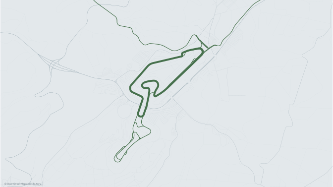
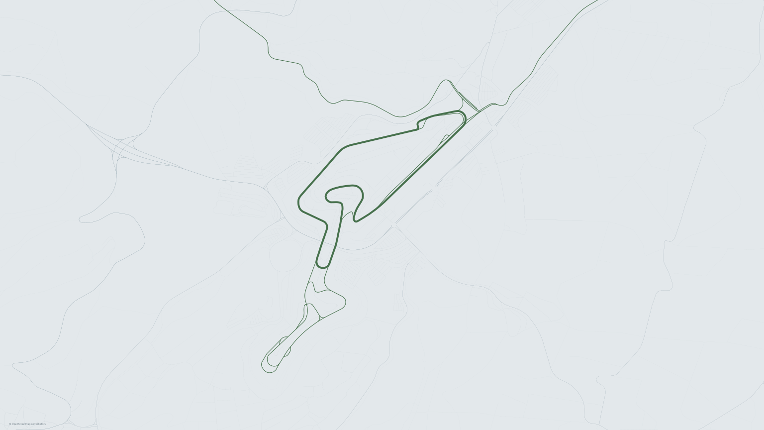
The name summary also reveals a compact layout stored across nine ways as Nürburgring Sprintstrecke. Keep only the nearby road network for context, with its line widths subdued so the Sprintstrecke remains the focus.

sprintstrecke <- raceways |>
  filter(raceway_name == "Nürburgring Sprintstrecke")

stopifnot(nrow(sprintstrecke) > 0)

sprint_bbox_raw <- sf::st_bbox(sprintstrecke)
sprint_centre <- c(
  (sprint_bbox_raw[["xmin"]] + sprint_bbox_raw[["xmax"]]) / 2,
  (sprint_bbox_raw[["ymin"]] + sprint_bbox_raw[["ymax"]]) / 2
)

# A slightly tighter frame makes the Sprintstrecke larger; shift south to move it up.
sprint_centre <- sprint_centre + c(0, -150)
sprint_frame <- make_frame(4500, 4500 / screen_ratio, sprint_centre)
sprint_bbox <- sf::st_bbox(sprint_frame)

sprint_roads <- sf::st_intersection(roads_surroundings, sprint_frame) |>
  mutate(sprint_width = line_width * 0.35)

sprint_map <- ggplot() +
  geom_sf(
    data = sprint_roads,
    aes(colour = line_colour, linewidth = sprint_width),
    lineend = "round"
  ) +
  geom_sf(
    data = sprintstrecke,
    colour = forest_green,
    linewidth = 1.35,
    lineend = "round",
    inherit.aes = FALSE
  ) +
  scale_colour_identity() +
  scale_linewidth_identity() +
  map_credit(bounds = sprint_bbox) +
  map_theme +
  coord_sf(
    crs = 25832,
    xlim = sprint_bbox[c("xmin", "xmax")],
    ylim = sprint_bbox[c("ymin", "ymax")],
    expand = FALSE,
    datum = NA
  )

sprint_map

The Nürburgring Sprintstrecke in forest green, surrounded by a subdued local road network.

Nürburgring Sprintstrecke highlighted within the nearby road network.

Export plots

Save the maps built through the post as PNG and SVG. The PNGs use the exact screen dimensions through ggsave(); SVG stays scalable.

images_dir <- "images"
dir.create(images_dir, recursive = TRUE, showWarnings = FALSE)

# Pixel dimensions fix the PNG size; dpi controls the physical scale used for styling.
save_map <- function(map, name) {
  ggsave(
    filename = file.path(images_dir, paste0(name, ".png")),
    plot = map,
    width = screen_width_px,
    height = screen_height_px,
    units = "px",
    dpi = export_dpi,
    # Use the map's own background for an opaque, edge-to-edge export.
    bg = NULL
  )

  ggsave(
    filename = file.path(images_dir, paste0(name, ".svg")),
    plot = map,
    width = screen_width_px,
    height = screen_height_px,
    units = "px",
    dpi = export_dpi,
    bg = NULL
  )
}

save_map(uniform_map, "roads-uniform")
save_map(width_map, "roads-hierarchy")
save_map(surroundings_map, "roads-surroundings")
save_map(detail_map, "roads-light")
save_map(dark_map, "roads-dark")
save_map(p_sections, "circuit-sections")
save_map(sprint_map, "sprintstrecke")

Preview version

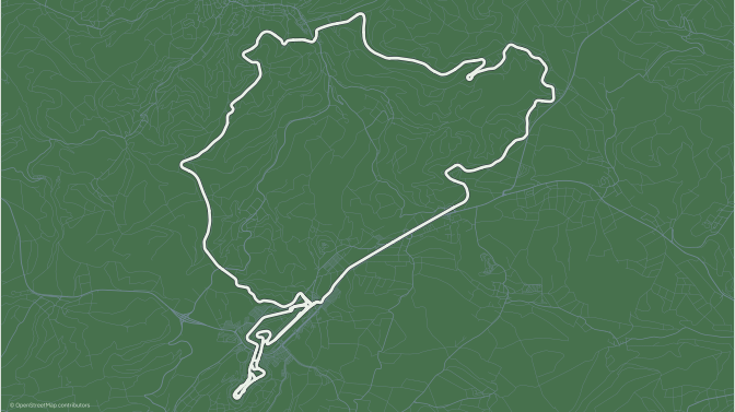
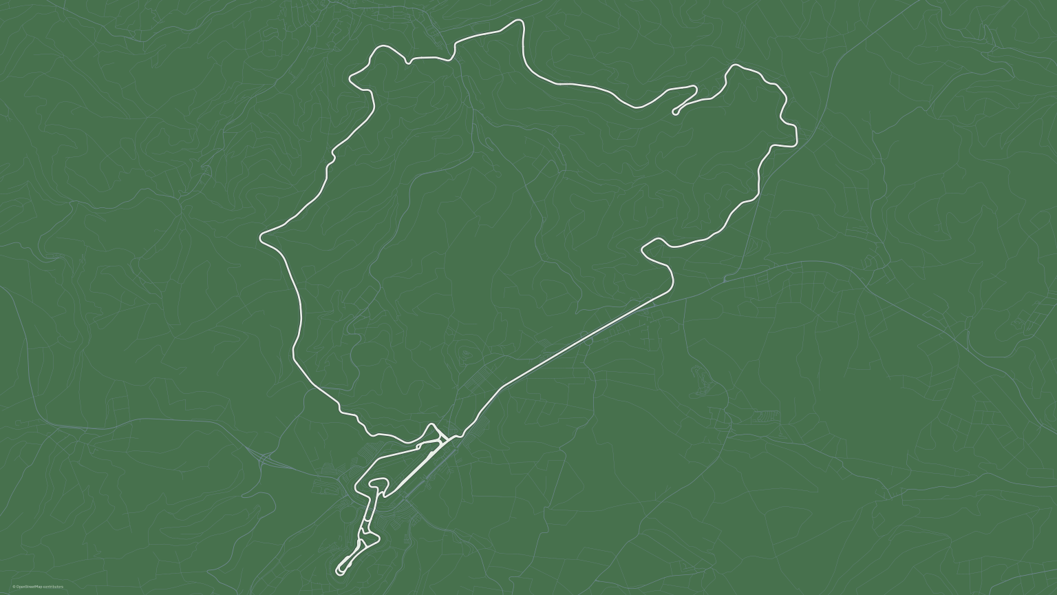
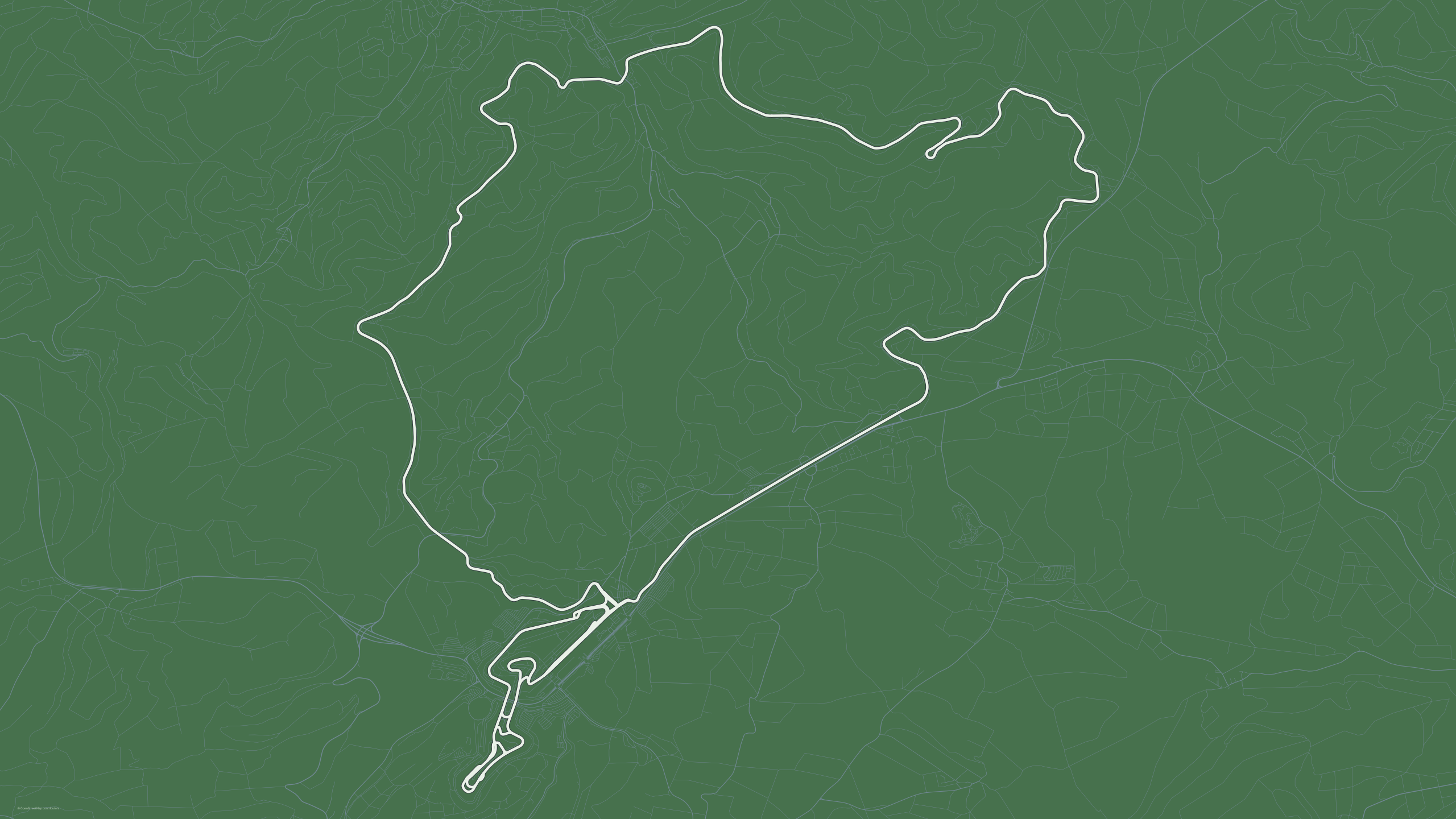
The blog preview uses a tighter frame. Nearby roads stay as a single quiet layer, while the circuit gets a two-stroke cartographic casing: a dark outer line and a narrower pale line. This keeps the GP complex legible without giving every road a heavy border.

# Reuse the same centre with a tighter frame, without measuring clipped roads again.
preview_bbox <- make_frame(
  visible_width_m,
  visible_height_m,
  map_centre
) |>
  sf::st_bbox()

# Keep context roads thin and uncased; reserve the stronger treatment for the circuit.
preview_context <- roads_context |>
  mutate(preview_width = pmax(line_width, 0.10))

preview_map <- ggplot() +
  geom_sf(
    data = preview_context,
    aes(linewidth = preview_width),
    colour = "#718894",
    lineend = "round"
  ) +
  # Draw the circuit twice: a dark casing first, then a narrower pale stroke.
  geom_sf(
    data = raceways,
    colour = asphalt_dark,
    linewidth = 1.35,
    lineend = "round",
    inherit.aes = FALSE
  ) +
  geom_sf(
    data = raceways,
    colour = "#EAF1E8",
    linewidth = 0.95,
    lineend = "round",
    inherit.aes = FALSE
  ) +
  scale_linewidth_identity() +
  map_credit(bounds = preview_bbox, colour = "#D3E0D1") +
  coord_sf(
    crs = 25832,
    xlim = preview_bbox[c("xmin", "xmax")],
    ylim = preview_bbox[c("ymin", "ymax")],
    expand = FALSE,
    datum = NA
  ) +
  map_theme +
  theme(
    panel.background = element_rect(fill = forest_green, colour = NA),
    plot.background = element_rect(fill = forest_green, colour = NA),
    plot.margin = margin(0, 0, 0, 0)
  )

preview_map

# Use the same base name for the blog card PNG and its scalable SVG counterpart.
save_map(preview_map, "preview")

SVG downloads: Uniform roads · Road hierarchy · Surroundings · Light version · Dark version · Circuit sections · Sprintstrecke · Preview

Data: © OpenStreetMap contributors, licensed under the ODbL.

Circuit and section reference: official Nürburgring Nordschleife guide.

Reference: Bastián Olea’s tutorial and its source code.