library(sf)
# Published longitude/latitude used only to locate the raceway ways.
search_lon <- 6.9476
search_lat <- 50.3356
# This generous window is used only to find the circuit around the search point.
search_width_km <- 14
# The final frame follows the circuit bounds and keeps a landscape proportion.
screen_ratio <- 16 / 9
terrain_margin_pct <- 12
# ETRS89 / UTM zone 32N gives this region coordinates in metres.
search_centre_utm <- sf::st_sfc(
sf::st_point(c(search_lon, search_lat)),
crs = 4326
) |>
sf::st_transform(25832)
search_centre_xy <- sf::st_coordinates(search_centre_utm)[1, ]
search_half_m <- search_width_km * 1000 / 2
# This broad square finds the circuit; it is not the terrain shown in the map.
search_frame_utm <- sf::st_bbox(
c(
xmin = search_centre_xy[[1]] - search_half_m,
ymin = search_centre_xy[[2]] - search_half_m,
xmax = search_centre_xy[[1]] + search_half_m,
ymax = search_centre_xy[[2]] + search_half_m
),
crs = sf::st_crs(25832)
) |>
sf::st_as_sfc()
search_bbox_wgs84 <- search_frame_utm |>
sf::st_transform(4326) |>
sf::st_bbox()The 2D Nürburgring post draws the circuit as a sequence of ggplot2 layers. This companion starts with the same OpenStreetMap geometry, but gives it a terrain surface. The result has two uses: a small WebGL model to rotate in the browser, and a white-background image suitable for the post or a card.
We will keep the first version deliberately short: choose the area, cache the data, shade the elevation and draw the circuit on top. The data download happens only when the local cache is absent, so camera and style experiments remain fast.
Data
The racetrack, not an arbitrary bounding box, defines the final frame. A small margin leaves enough surrounding relief to read the circuit in context.
We use the coordinates listed for the Nürburgring only as a search seed. A line’s length does not determine its geographic footprint, so we do not try to infer the circuit’s width from its lap distance. Instead, a deliberately generous 14 km square retrieves the nearby raceway ways. Once OpenStreetMap returns those geometries, their measured bounds define the frame we actually plot. The 16:9 ratio and 12% margin are visual choices for this post.
Download once, then reuse locally
On its first run this chunk gets the raceway from OpenStreetMap and the elevation from AWS terrain tiles through elevatr. It stores the processed geometry, elevation matrix and extent in the post’s data/ directory. Commit that RDS with the post: subsequent renders will read it instead of making either network request.
Download and cache the terrain data
library(dplyr)
library(osmdata)
library(terra)
cache_file <- "blog/posts/2026-09-29-nurburgring-in-3d-with-rayshader/data/nurburgring-3d.rds"
cache_version <- 2L
terrain_data <- if (file.exists(cache_file)) readRDS(cache_file) else NULL
cache_is_current <- !is.null(terrain_data$cache_version) &&
terrain_data$cache_version == cache_version
if (!cache_is_current) {
# Query ways only: nodes and relations are not used for the circuit line.
raceway_query <- osmdata::opq(
bbox = search_bbox_wgs84,
osm_types = "way",
timeout = 180
) |>
osmdata::add_osm_feature(key = "highway", value = "raceway")
# Overpass is public infrastructure, so retry a small set of global mirrors.
download_raceways <- function(query) {
overpass_urls <- c(
"https://overpass.kumi.systems/api/interpreter",
"https://overpass-api.de/api/interpreter",
"https://api.openstreetmap.fr/oapi/interpreter"
)
original_url <- osmdata::get_overpass_url()
on.exit(osmdata::set_overpass_url(original_url), add = TRUE)
errors <- character()
for (overpass_url in overpass_urls) {
osmdata::set_overpass_url(overpass_url)
message("Requesting raceway data from ", overpass_url, "...")
response <- tryCatch(
osmdata::osmdata_sf(query, quiet = TRUE),
error = function(error) error
)
if (!inherits(response, "error")) {
return(response)
}
errors <- c(errors, conditionMessage(response))
}
stop(
"All selected Overpass mirrors failed. Try rendering again later. Last error: ",
tail(errors, 1)
)
}
track <- download_raceways(raceway_query)$osm_lines |>
filter(highway == "raceway") |>
select(osm_id, name, geometry) |>
sf::st_transform(25832) |>
sf::st_intersection(search_frame_utm)
if (nrow(track) == 0) {
stop("No raceway geometry found around the Nürburgring search area.")
}
# Expand the circuit bounds, adjusting the shorter side to the output ratio.
track_bbox <- sf::st_bbox(track)
frame_width_m <- (track_bbox[["xmax"]] - track_bbox[["xmin"]]) *
(1 + terrain_margin_pct / 100)
frame_height_m <- (track_bbox[["ymax"]] - track_bbox[["ymin"]]) *
(1 + terrain_margin_pct / 100)
if (frame_width_m / frame_height_m < screen_ratio) {
frame_width_m <- frame_height_m * screen_ratio
} else {
frame_height_m <- frame_width_m / screen_ratio
}
track_centre <- c(
mean(track_bbox[c("xmin", "xmax")]),
mean(track_bbox[c("ymin", "ymax")])
)
terrain_frame_utm <- sf::st_bbox(
c(
xmin = track_centre[[1]] - frame_width_m / 2,
ymin = track_centre[[2]] - frame_height_m / 2,
xmax = track_centre[[1]] + frame_width_m / 2,
ymax = track_centre[[2]] + frame_height_m / 2
),
crs = sf::st_crs(25832)
) |>
sf::st_as_sfc()
terrain_bbox_wgs84 <- terrain_frame_utm |>
sf::st_transform(4326) |>
sf::st_bbox()
# elevatr needs two corners to identify the terrain tiles covering the frame.
elev_locations <- data.frame(
x = c(terrain_bbox_wgs84[["xmin"]], terrain_bbox_wgs84[["xmax"]]),
y = c(terrain_bbox_wgs84[["ymin"]], terrain_bbox_wgs84[["ymax"]])
)
dem <- elevatr::get_elev_raster(
locations = elev_locations,
z = 13,
prj = "EPSG:4326",
src = "aws",
verbose = TRUE
) |>
terra::rast() |>
terra::project("EPSG:25832", method = "bilinear")
# Cropping after projection makes the saved terrain match the circuit frame.
dem <- terra::crop(dem, terra::ext(terra::vect(terrain_frame_utm)))
elevation <- rayshader::raster_to_matrix(dem)
terrain_extent <- as.vector(terra::ext(dem))
names(terrain_extent) <- c("xmin", "xmax", "ymin", "ymax")
dir.create(dirname(cache_file), recursive = TRUE, showWarnings = FALSE)
saveRDS(
list(
cache_version = cache_version,
track = track,
elevation = elevation,
extent = terrain_extent,
resolution_m = mean(terra::res(dem))
),
cache_file
)
terrain_data <- readRDS(cache_file)
}
track <- terrain_data$track
elevation <- terrain_data$elevation
terrain_extent <- terrain_data$extent
resolution_m <- terrain_data$resolution_m
# The overlay generator expects individual LINESTRING geometries.
track_paths <- track |>
sf::st_cast("LINESTRING", warn = FALSE)The track
Let’s start with track. It is an sf data frame: two ordinary columns, osm_id and name, plus a geometry column with the lines. Printing it tells us how many features we have, their geometry type, bounding box and coordinate reference system.
dplyr::glimpse(track)Rows: 98
Columns: 3
$ osm_id <chr> "26543901", "27852583", "27852990", "30815119", "31009257", "…
$ name <chr> "Anbindung zur Nordschleife", "Anbindung zum GP Kurs", "Nürbu…
$ geometry <LINESTRING [m]> LINESTRING (354062.3 557819..., LINESTRING (354207…utils::head(track, 6)Simple feature collection with 6 features and 2 fields
Geometry type: LINESTRING
Dimension: XY
Bounding box: xmin: 353133 ymin: 5577439 xmax: 354305.5 ymax: 5578268
Projected CRS: ETRS89 / UTM zone 32N
osm_id name geometry
26543901 26543901 Anbindung zur Nordschleife LINESTRING (354062.3 557819...
27852583 27852583 Anbindung zum GP Kurs LINESTRING (354207.3 557818...
27852990 27852990 Nürburgring Sprintstrecke LINESTRING (353281 5577439,...
30815119 30815119 Boxengasse LINESTRING (353919.7 557816...
31009257 31009257 Boxengasse an T13 LINESTRING (354305.5 557822...
31010602 31010602 Variante 24h-Rennen LINESTRING (353458.9 557755... west_to_east_km south_to_north_km
6.12 6.32 So this is not one continuous circuit line. OpenStreetMap stores the circuit, its named sections and connecting roads as separate ways. They are already projected to EPSG:25832, which means their coordinates are measured in metres. Together the returned raceway features occupy a little more than 6 km in each direction. The 14 km discovery square was deliberately generous; from this point onward, these measured bounds replace it and define the terrain frame.
Before doing anything in 3D, let’s plot those lines. Nothing fancy yet: this is only a quick check that we downloaded the geometry we expected.
plot(sf::st_geometry(track), axes = TRUE, asp = 1)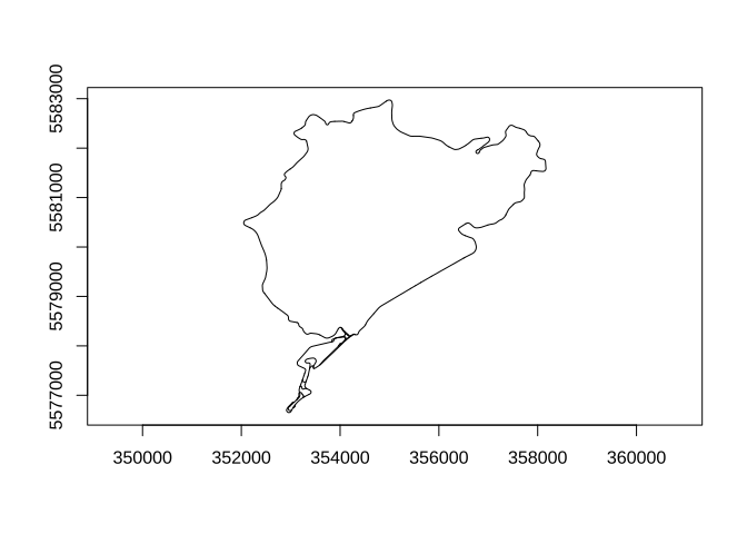
The elevation matrix
The other main object is elevation. This time we do not have a data frame or an sf object, but a numeric matrix created by rayshader::raster_to_matrix(). Every cell contains one terrain height in metres. Let’s look at its structure and range.
str(elevation) num [1:2062, 1:1160] 375 374 374 373 373 ... minimum_m maximum_m resolution_m
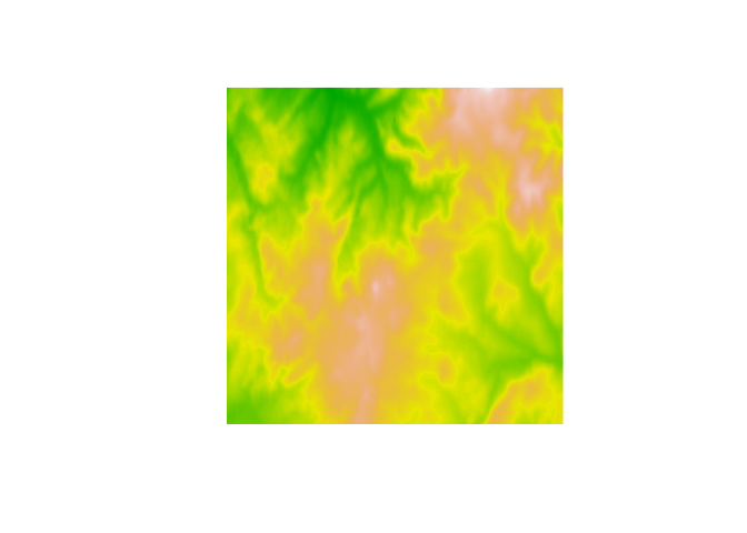
302.0 706.0 6.1 A matrix is already enough to get a first look at the terrain. We use image() instead of plot(): the latter would interpret the first two matrix columns as paired coordinates. Reversing the columns restores the north-up orientation of the original raster.
image(
elevation[, ncol(elevation):1],
col = grDevices::terrain.colors(64),
axes = FALSE,
asp = 1,
useRaster = TRUE
)
Where is the matrix?
There is one piece missing. A matrix has rows, columns and values, but it does not know where it is on a map. terrain_extent is a named numeric vector with its projected limits: xmin, xmax, ymin and ymax. resolution_m is simply the average ground size of one cell. Together they tell rayshader where the sf lines belong on the elevation matrix.
terrain_extent xmin xmax ymin ymax
348817.5 361400.4 5576270.5 5583349.1 resolution_m[1] 6.102247The initial request downloads only the AWS Terrain Tiles that cover this small frame, through elevatr, not a global elevation dataset. The RDS is then a processed cache rather than a copy of every raw response: it keeps track, elevation, terrain_extent and resolution_m. A cache fixed at the final 400-cell limit would be smaller, but keeping the full matrix lets us change that resolution without downloading the terrain again. The next step creates a lighter working surface for both the WebGL model and the rendered images.
Build and explore the terrain
The full matrix stays in the cache, but the 3D scene does not need every cell. Rather than preparing the complete texture in one long pipeline, let’s build it one layer at a time and look at each result.
A lighter height matrix
First we sample a smaller working matrix. interactive_step tells us how many cells we skip in each direction. This makes the scene faster, but also increases the ground distance represented by every remaining cell.
library(rayshader)
# Limit the working surface while keeping the full elevation matrix in the cache.
interactive_max_dim <- 600
# Downsample the working mesh, retaining the full matrix in the local cache.
interactive_step <- max(1L, ceiling(max(dim(elevation)) / interactive_max_dim))
interactive_rows <- seq.int(1L, nrow(elevation), by = interactive_step)
interactive_cols <- seq.int(1L, ncol(elevation), by = interactive_step)
elevation_interactive <- elevation[
interactive_rows,
interactive_cols,
drop = FALSE
]
interactive_resolution_m <- resolution_m * interactive_step
# A smaller zscale exaggerates the vertical relief in rayshader.
vertical_exaggeration <- 2
zscale <- interactive_resolution_m / vertical_exaggeration
c(
original_grid = paste(dim(elevation), collapse = " × "),
working_grid = paste(dim(elevation_interactive), collapse = " × "),
keep_every_nth_cell = interactive_step,
working_resolution_m = round(interactive_resolution_m, 1)
) original_grid working_grid keep_every_nth_cell
"2062 × 1160" "516 × 290" "4"
working_resolution_m
"24.4" zscale compares that horizontal cell spacing with the vertical values. Dividing it by two exaggerates the relief: this is a visual choice rather than a change to the elevation data.
Give the terrain an organic palette
height_shade() turns the numeric matrix into an RGB image. Dark greens describe the lower elevations, while olive, earth and mineral tones appear progressively higher. This gives the surface an organic reading without downloading satellite imagery or pretending that the colours describe actual land cover.
# These colours suggest forest, earth and exposed terrain without claiming to be
# a satellite or vegetation map.
organic_palette <- grDevices::colorRampPalette(c(
"#25382E",
"#40513A",
"#687052",
"#8A795B",
"#C7BA96"
))(256)
terrain_texture <- elevation_interactive |>
rayshader::height_shade(texture = organic_palette)
rayshader::plot_map(terrain_texture)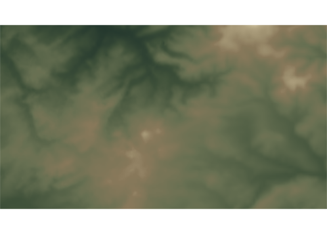
Add directional light
ray_shade() follows the light across the elevation matrix, so a ridge can cast a shadow on the terrain behind it. The light comes from 315° and sits 35° above the horizon. We keep the darkening subtle: the goal is to reveal the relief, not turn every valley black.
terrain_shadow <- rayshader::ray_shade(
elevation_interactive,
zscale = zscale,
sunangle = 315,
sunaltitude = 35
)
# Values closer to one retain more of the original palette.
terrain_texture <- terrain_texture |>
rayshader::add_shadow(terrain_shadow, max_darken = 0.70)
rayshader::plot_map(terrain_texture)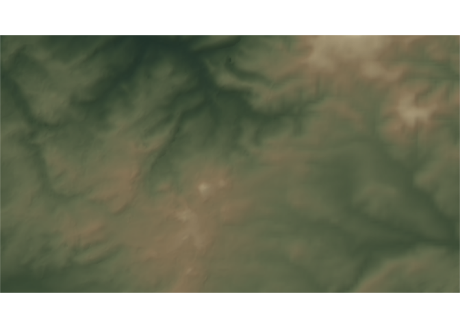
Draw the track on the texture
generate_line_overlay() translates the projected sf lines into an RGBA image aligned with the elevation matrix. RGBA means red, green, blue and alpha, the transparency channel. It is therefore an image array, not a vector of values. Calling base plot() on it flattens the channels and produces a misleading index plot; plot_map() understands the image structure.
We first draw a wide dark line. resolution_multiply = 2 creates the overlay at twice the working resolution so its edges remain crisp.
track_casing_overlay <- rayshader::generate_line_overlay(
track_paths,
extent = terrain_extent,
heightmap = elevation_interactive,
resolution_multiply = 2,
color = "#202724",
linewidth = 7
)
list(
class = class(track_casing_overlay),
dimensions = dim(track_casing_overlay)
)$class
[1] "rayimg" "array"
$dimensions
[1] 580 1032 4Add that array to the shaded terrain and use plot_map() to inspect the actual image composition.
terrain_with_casing <- terrain_texture |>
rayshader::add_overlay(
track_casing_overlay,
rescale_original = TRUE
)
rayshader::plot_map(terrain_with_casing)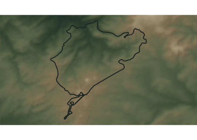
The second overlay is narrower and concrete grey. Placing it over the dark line creates a simple two-stroke track that remains visible on both light and shaded slopes without looking painted white.
track_line_overlay <- rayshader::generate_line_overlay(
track_paths,
extent = terrain_extent,
heightmap = elevation_interactive,
resolution_multiply = 2,
color = "#C4C6C2",
linewidth = 4
)
terrain_texture <- terrain_with_casing |>
rayshader::add_overlay(track_line_overlay, rescale_original = TRUE)
rayshader::plot_map(terrain_texture)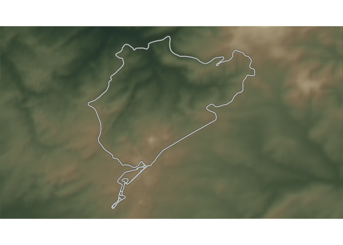
Explore the model
The track is already part of terrain_texture, so plot_3d() only needs to wrap that finished image over the elevation matrix. Drawing the paths again in 3D would duplicate the line and expose the joins between the original OpenStreetMap ways.
The 2D checks above remain north-up. For the editorial 3D view, we rotate the camera 30° so the terrain follows the diagonal of the wide frame and uses more of the available space. This changes only the presentation: phi sets the camera elevation and fov supplies the perspective.
The theta, phi, zoom and fov arguments control the viewpoint; they are not properties of the Nürburgring. We choose them here and reuse the same camera for the interactive and static versions.
# A small clockwise rotation lets the rectangular terrain fill the wide frame.
camera_theta <- 330
camera_phi <- 42
camera_zoom <- 0.65
camera_fov <- 35Build the interactive scene
# This helper recreates the same terrain for the widget and both image exports.
draw_terrain_scene <- function() {
terrain_texture |>
rayshader::plot_3d(
elevation_interactive,
zscale = zscale,
theta = camera_theta,
phi = camera_phi,
zoom = camera_zoom,
fov = camera_fov,
windowsize = c(1200, 675),
background = "#D7D9D5",
solid = TRUE,
solidcolor = "#45483F",
solidlinecolor = "#34372F",
shadow = TRUE,
shadowcolor = "#77786F"
)
}
draw_terrain_scene()
rgl::rglwidget(width = 1200, height = 675)