h|1i|0g|3h|2c|1h|2a|1r|3t|2e|1r|2{userchile}
Joshua Kunst, Julio 2017
Advertencia
Todos los gráficos de , 3D y la combinación de estos en esta presentación son ilustrativos y no representan el estilo ni el gusto de quien lo presenta
Quien soy y que haré(mos)
Quien soy
- De día hago como que trabajo en riesgo (70%)
- En Proyectos Personales (30%)
- Me gusta escribir código (en R)
- Y compartirlo en jkunst.com
- De casualidad soy Estadístico . Así mismo useR
Que haremos
- Revisar formas de visualizar en R
- Qué es highcharts?
- Cómo usar highcharter?
- Función genérica
hchart - Ejemplos simples, y quizás algunos más complejos. Integración con
shiny,rmarkdown. Si el tiempo da
Por que lo haríamos?
- La visualización ayuda a descubrir y explicar
- En muchos casos resume un gran desarrollo que hemos hecho
- Y bueno, en general es mejor recibido si es claro y atractivo

Historia
R base
Haciendo visualizaciones desde 2000 AC
y <- rpois(100, lambda = 3)
plot(table(y))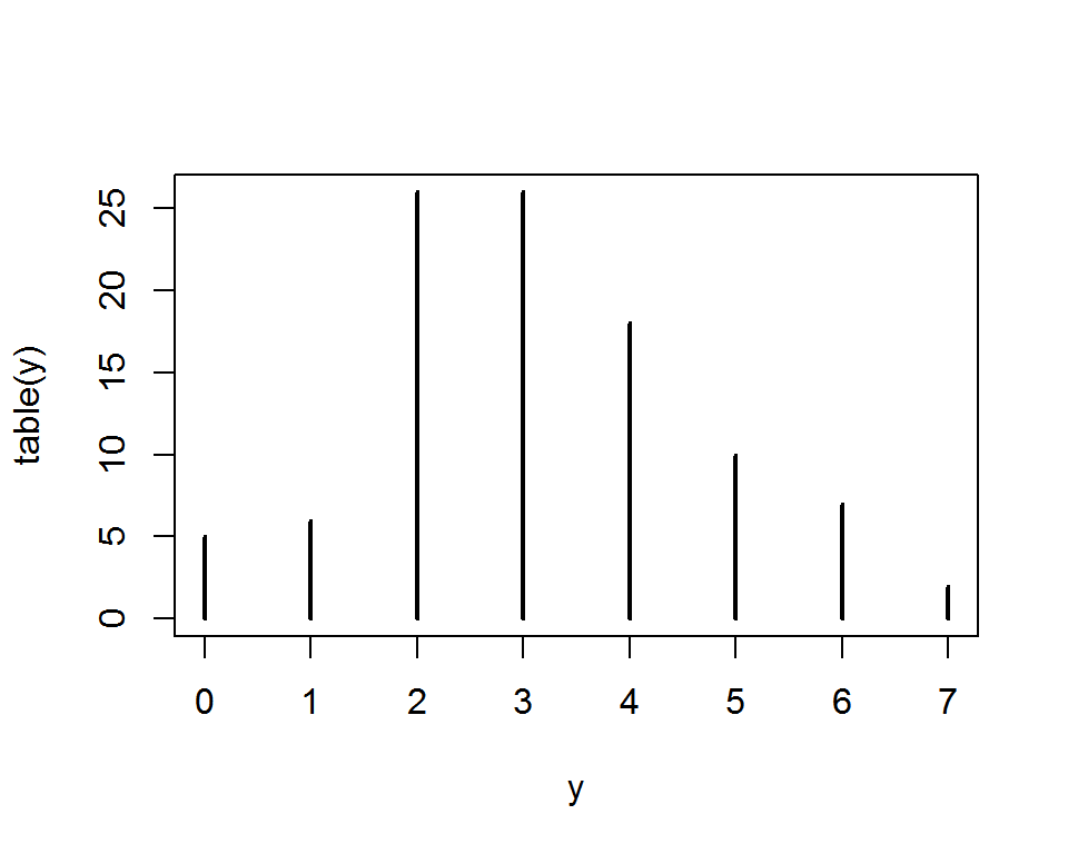
R base
Rápido para hacer cosas simples, pero no escala de la mejor manera.
plot(AirPassengers)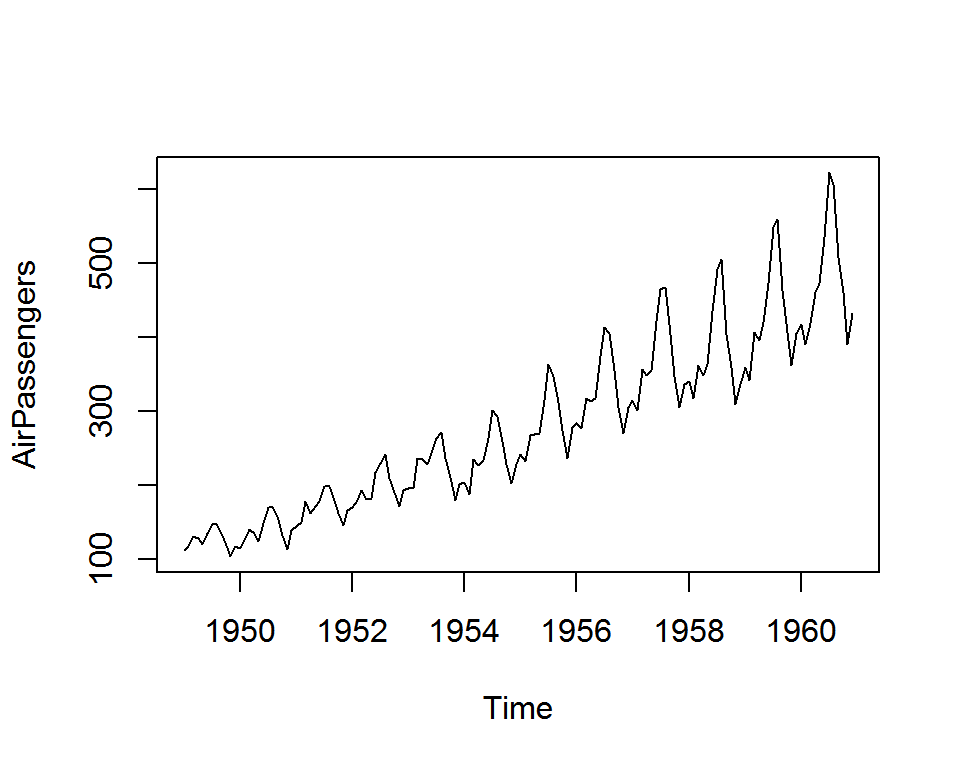
ggplot2 & Lattice
latticebasado en trellisggplot2basado en gramar of graphics- Paquetes con buen soporte en datos multivariados (colores, facets, …)
ggplot2es el rey de los gráficos estáticos- Muy flexible dado que existe la posibilidad de crear extensiones + temas
htmlwidgets
- Surgió como la 2da iteración de
rChartspara graficar usando librerías de javascript (basadas en web). - Permite a usuarios
abusar de estás librerías sin necesariamente conocer js - Provee un framework -una estandarización- para que un desarrollador porte una librería javascript a R
- Una librería basada en
htmlwidgetsvieneshiny&rmarkdownready
htmlwidgets
Para la mayoría de las librerías sueltas en la web existe un paquete para R
Consideraciones
R es muy flexible lo que lleva a:
- Tener gran variedad de opciones
- Considerar que cada paquete tiene su propia sintaxis
- Peeero siempre estarás acompañado de la buena comunidad que R posee
highcharts
Highcharts
- highcharts es una popular -entre otras- librería de javascript de visualización
- Muy
viejamadura y flexible. Muchos plugins! - Muchos tipos de gráficos, incluyendo financieros y mapas
- highcharter es un poco más que el wrapper highcharts para R. Por lo que hereda todas sus características. Yay!
Como luce un highcharts
Highcharts Demo
Highcharts API
highchartrs en R
Highcharts en R
- highcharter implementa todas los atributos como funciones
hc_* - Por ej: para el titulo (
title) se debe usarhc_title()y así… - ¿Los parámetros? de la API http://api.highcharts.com/highcharts
- Por lo que para partir: buscas, ves el ejemplo, y luegos implementas en R.
Inicializando
# install.package("highcharter")
# source("https://install-github.me/jbkunst/highcharter")
library(highcharter)
hc <- highchart()
hc
Títulos y subtítulos
hc <- hc %>%
  hc_title(text = "Stock") %>%
  hc_subtitle(text = "Fuente: Imaginación")
hc
Agregando data
ventas <- abs(1:12 + rnorm(12) + 2)
hc <- hc %>%
  hc_add_series(data = ventas, name = "Ventas")
hc
Agregando más data
ventas2 <- abs(ventas*.7 + rnorm(12, sd = 0.8))
hc <- hc %>%
  hc_add_series(data = ventas2, name = "Competencia")
hc
Configurando opciones
hc %>%
  hc_chart(
    type = "column", borderColor = '#EBBA95', borderRadius = 10, borderWidth = 3,
    options3d = list(enabled = TRUE, alpha = 15, beta = 15))
Configurando ejes
hc <- hc %>%
  hc_xAxis(categories = month.abb) %>%
  hc_yAxis(labels = list(format = "${value:.1f}"))
hc
Entonces
hcf <- highchart() %>%
  hc_title(text = "Stock") %>%
  hc_subtitle(text = "Fuente: Imaginación") %>%
  hc_add_series(data = ventas, name = "Ventas", color = "#3B5997",
                type = "area", fillOpacity = 0.15, lineWidth = 2)  %>%
  hc_add_series(data = ventas2, name = "Compentencia", visible = FALSE) %>%
  hc_xAxis(categories = month.abb) %>%
  hc_yAxis(labels = list(format = "${value:.1f}"), min = 0) %>%
  hc_tooltip(valueDecimals = 2, valuePrefix = "$", table = TRUE)
Entonces
Ehmmm…
- … Ok ok Todo puede ser muy bonito, pero requiere de mucho código… que lata!
- … Y que sucede si tengo 20 series? Una por una? Pff!

hchart al rescate
y otros atajos
hchart
- Función genérica, graficará algo dependiendo del tipo de objeto
- El mismo espíritu que
plot - La idea es tener algo boss/production-ready al instante
- Implementados series de tiempo, forecast, data.frames, PCA, dist, …
- Simplemente un
hchart(objeto)
hchart
x <- rnorm(1000)
hchart(x)
hchart
hchart(density(x), color = "skyblue", name = "Densidad!")hchart (+ bonus!)
library(forecast)
hchart(forecast(AirPassengers, h = 30)) %>%
  hc_exporting(enabled = TRUE)
hchart
hchart(princomp(USArrests, cor = TRUE))hchart
hchart(cor(mtcars))hchart en data.frames
data(economics, economics_long, package = "ggplot2")
print(economics, n = 3); print(economics_long, n = 3)
## # A tibble: 574 x 6
## date pce pop psavert uempmed unemploy
## <date> <dbl> <int> <dbl> <dbl> <int>
## 1 1967-07-01 507.4 198712 12.5 4.5 2944
## 2 1967-08-01 510.5 198911 12.5 4.7 2945
## 3 1967-09-01 516.3 199113 11.7 4.6 2958
## # ... with 571 more rows## # A tibble: 2,870 x 4
## # Groups: variable [5]
## date variable value value01
## <date> <fctr> <dbl> <dbl>
## 1 1967-07-01 pce 507.4 0.0000000000
## 2 1967-08-01 pce 510.5 0.0002660008
## 3 1967-09-01 pce 516.3 0.0007636797
## # ... with 2,867 more rowshchart en data.frames
hchart(economics_long, "line", hcaes(date, value01, group = variable)) %>%
  hc_tooltip(shared = TRUE, valueDecimals = 2)
hciconarray
hciconarray(c("auto", "camion", "avion"), c(40, 15, 10),
            icons = c("car", "truck", "plane"), size = 6)
hcmap
hcmap("countries/cl/cl-all")hcmap
data("USArrests", package = "datasets")
USArrests <- mutate(USArrests, "woe-name" = rownames(USArrests))

hcmap(map = "countries/us/us-all", data = USArrests,
      joinBy = "woe-name", value = "UrbanPop", name = "Urban Population")
Vamos al codear!
Gracias
Links de interés
- & jbkunst
- http://jkunst.com
- Highcharter devsite: https://github.com/jbkunst/highcharter
- Presentación: http://jkunst.com/r-material/201707-highcharter-en-una-cascara-de-nuez/
- Código: http://jkunst.com/r-material/201707-highcharter-en-una-cascara-de-nuez/code.html