Generating data set
The main function is sim_xy, you need to define:
- A number of observations to simulate.
- Values and .
- A distribution to sample
.
For example
stats::runiforpurrr::partial(stats::rnorm, mean = 5, sd = 1). - A function to sample error values like
purrr::partial(stats::rnorm, sd = 0.5).
library(klassets)
library(ggplot2)
library(patchwork)

set.seed(123)

df_default <- sim_xy()

df_default
#> # A tibble: 500 × 2
#>        x     y
#>    <dbl> <dbl>
#>  1  2.34  3.87
#>  2  2.36  3.68
#>  3  2.53  4.78
#>  4  2.69  4.72
#>  5  2.78  3.63
#>  6  2.84  4.37
#>  7  2.95  4.03
#>  8  2.95  3.44
#>  9  2.95  4.55
#> 10  2.99  4.45
#> # ℹ 490 more rows

plot(df_default)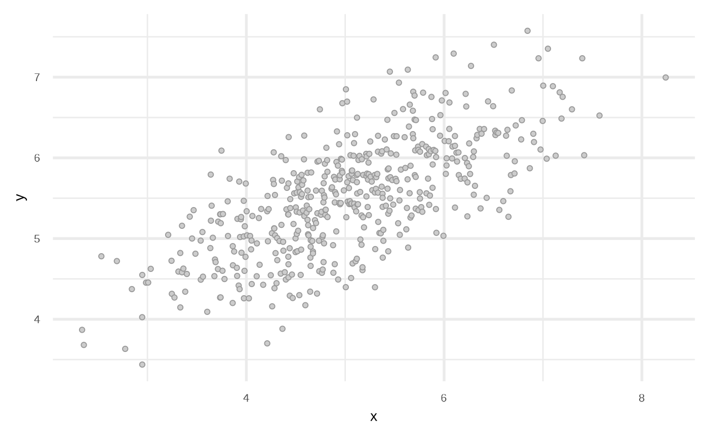
We can modify the data frame to get other types of relationships.
df <- sim_xy(n = 1000, x_dist = runif)

df <- dplyr::mutate(df, y = y + 2*sin(5 * x) + sin(10 * x))

plot(df)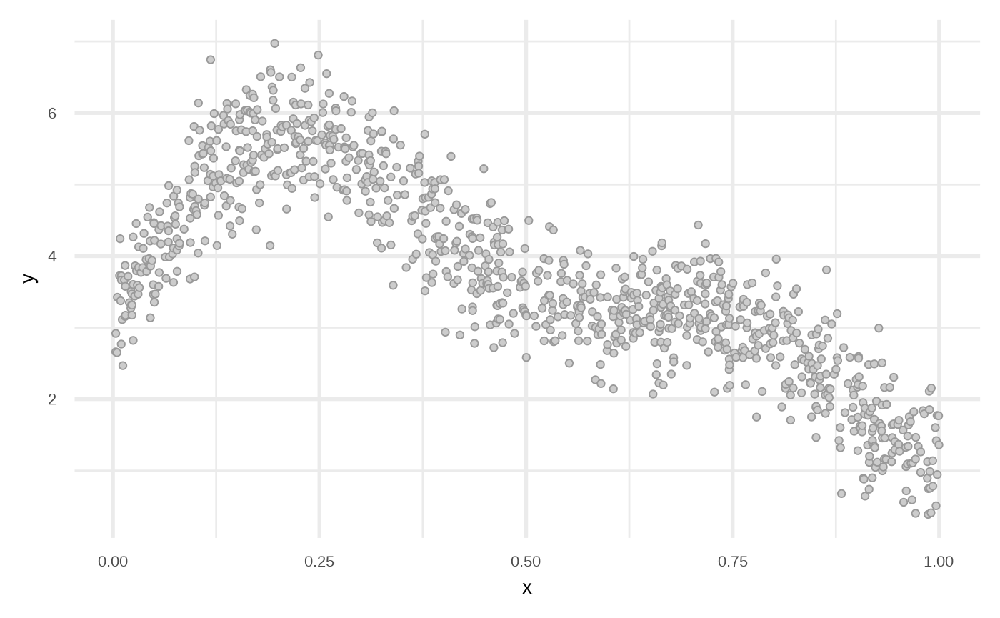
Fit regression algorithms
Linear Regression
This function uses stats::lm to fit a model.
df_lr <- fit_linear_model(df)

df_lr
#> # A tibble: 1,000 × 3
#>          x     y prediction
#>      <dbl> <dbl>      <dbl>
#>  1 0.00352  2.66       5.56
#>  2 0.00354  2.92       5.56
#>  3 0.00499  2.65       5.56
#>  4 0.00540  3.42       5.56
#>  5 0.00804  3.72       5.55
#>  6 0.00872  4.24       5.54
#>  7 0.00934  3.37       5.54
#>  8 0.0101   2.77       5.54
#>  9 0.0103   3.72       5.54
#> 10 0.0103   3.66       5.54
#> # ℹ 990 more rows

plot(df_lr)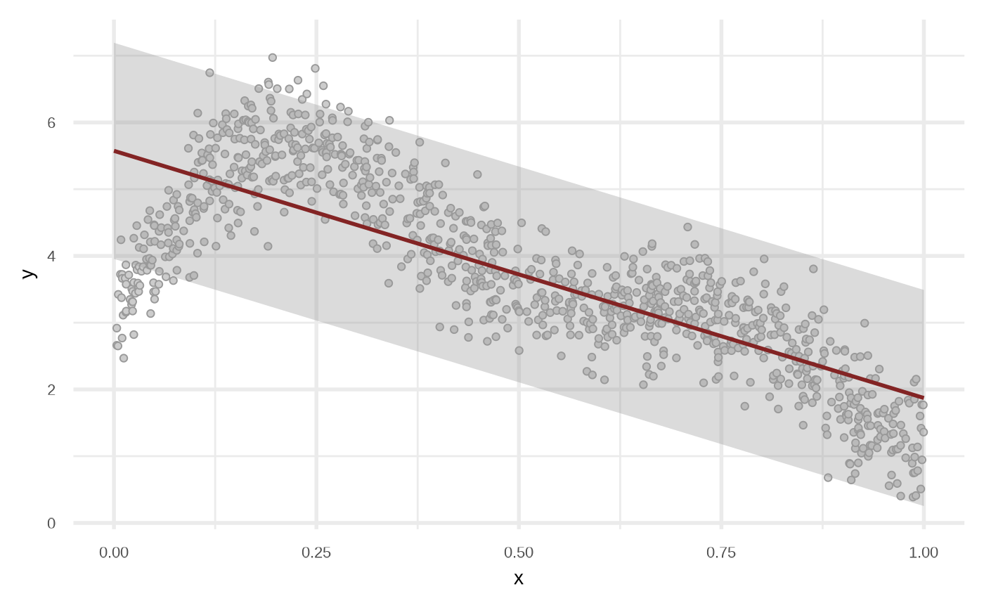
By default the model use order = 1 of the variables,
i.e, response ~ x + y. We can get a better fit if we
increase the order.
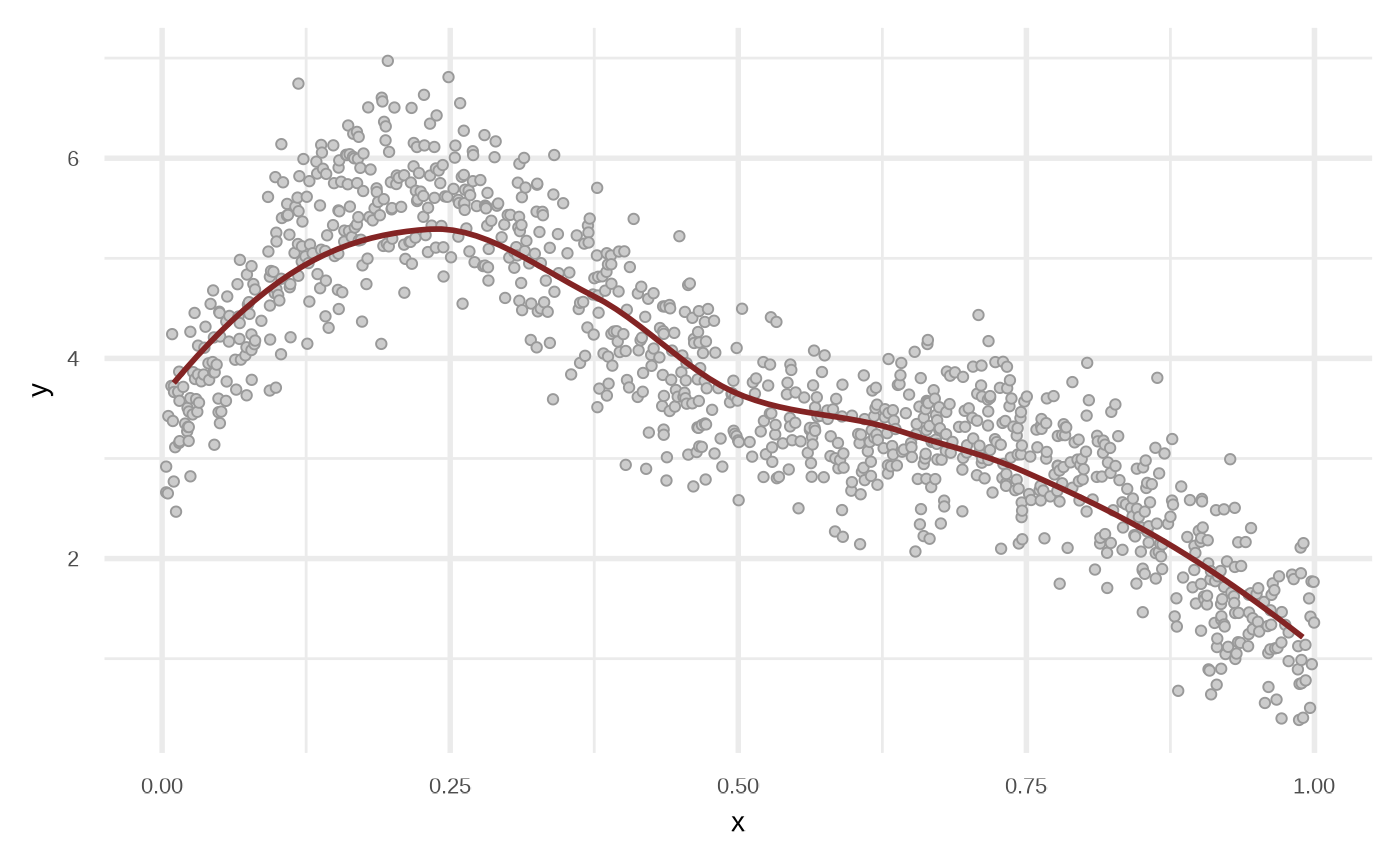
df_lr2 <- fit_linear_model(df, order = 4, stepwise = TRUE)

attr(df_lr2, "model")
#>
#> Call:
#> stats::lm(formula = y ~ x + x_2 + x_3 + x_4, data = df)
#>
#> Coefficients:
#> (Intercept)            x          x_2          x_3          x_4
#>       2.726       35.066     -137.903      186.228      -85.616

plot(df_lr2)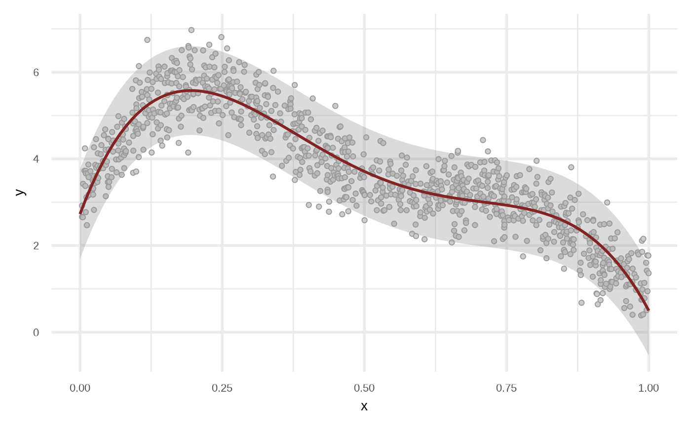
Testing various orders.
orders <- c(1, 2, 3, 4)

orders |>
  purrr::map(fit_linear_model, df = df) |>
  purrr::map(plot) |>
  purrr::reduce(`+`) +
  patchwork::plot_layout(guides = "collect") &
  theme_void() + theme(legend.position = "none")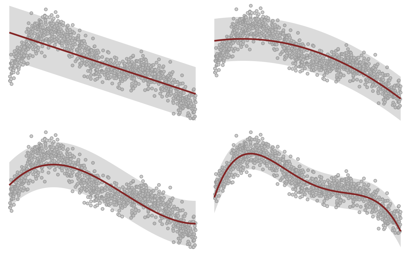
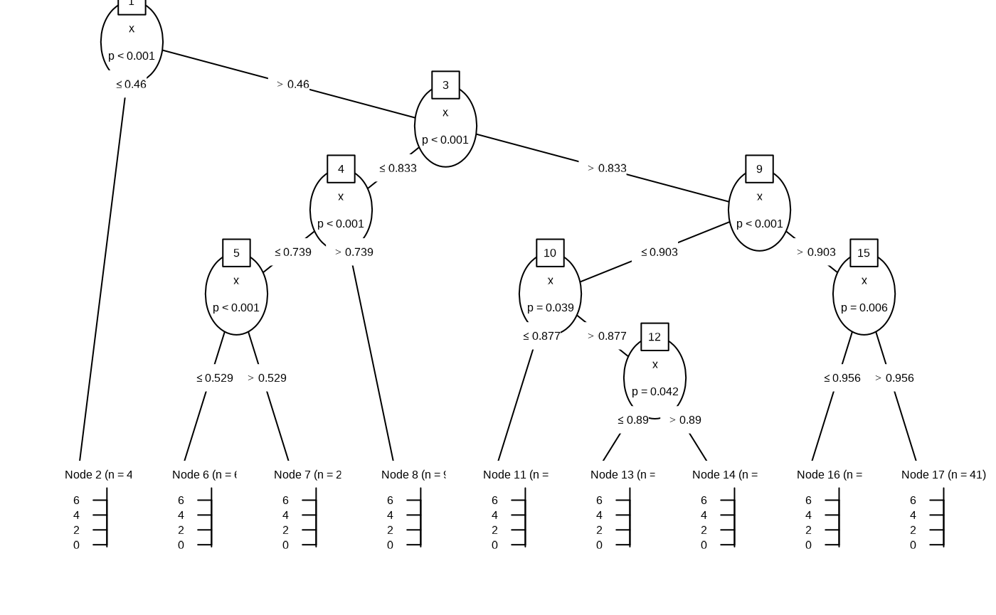
Regression Tree
Internally the functions uses partykit::ctree.
df_rt <- fit_regression_tree(df)

plot(df_rt)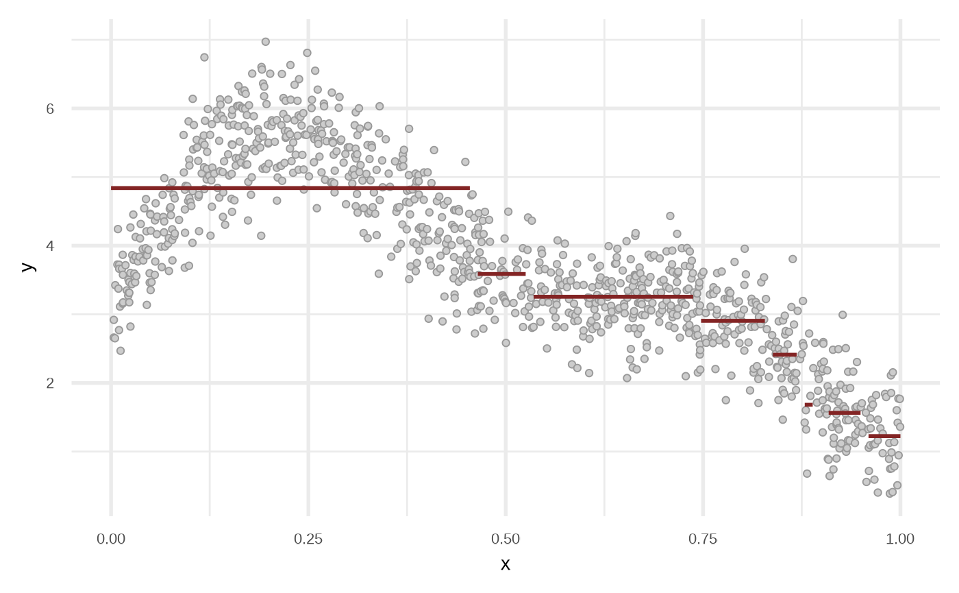
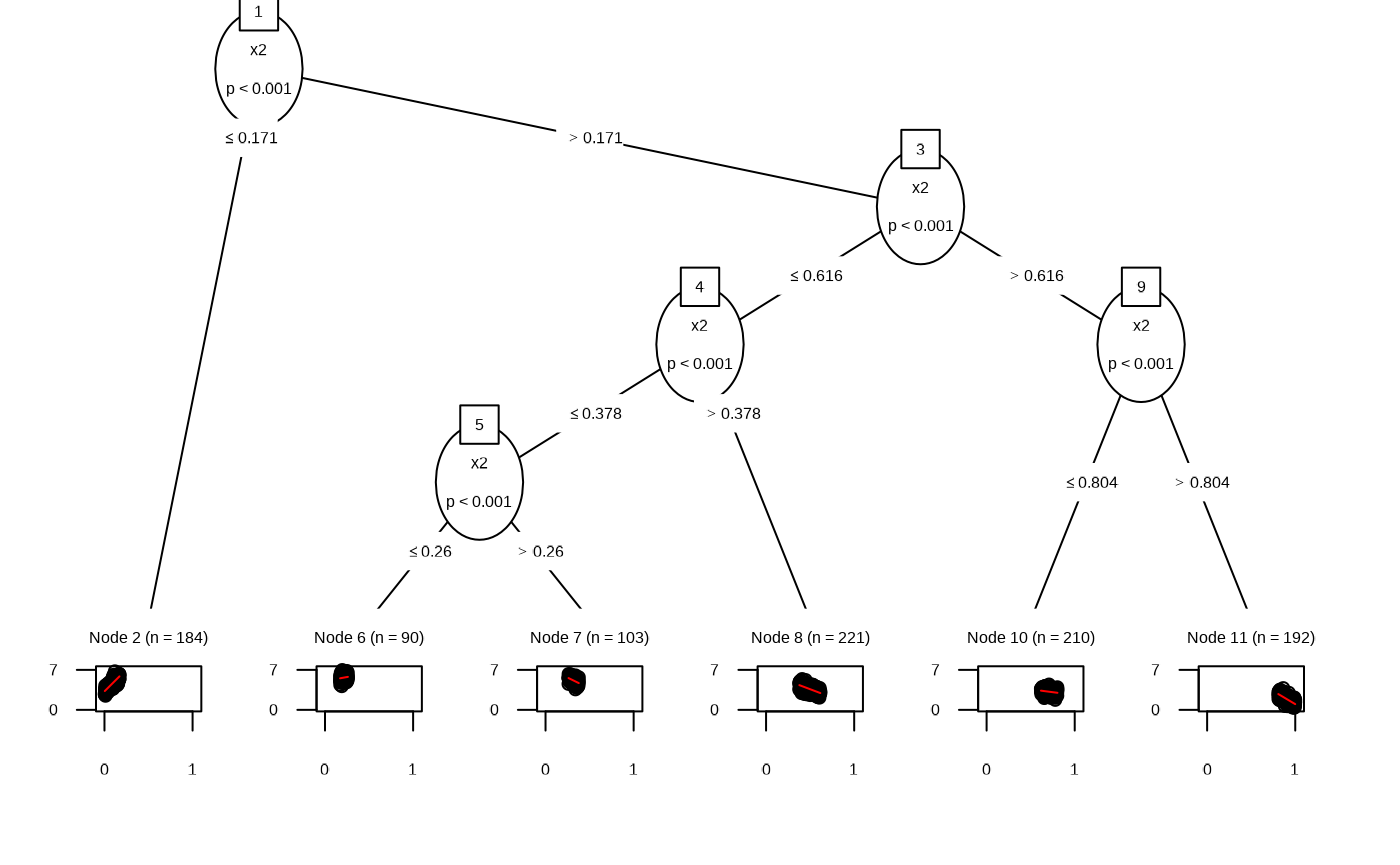
Linear Model Tree
Internally the functions uses partykit::mltree.
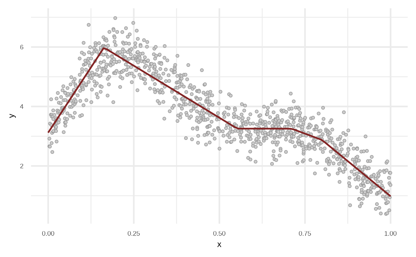
df_lmt <- fit_linear_model_tree(df)

plot(df_lmt)
Random Forest
Internally the functions uses partykit::cforest.
df_rf <- fit_regression_random_forest(df)

plot(df_rf)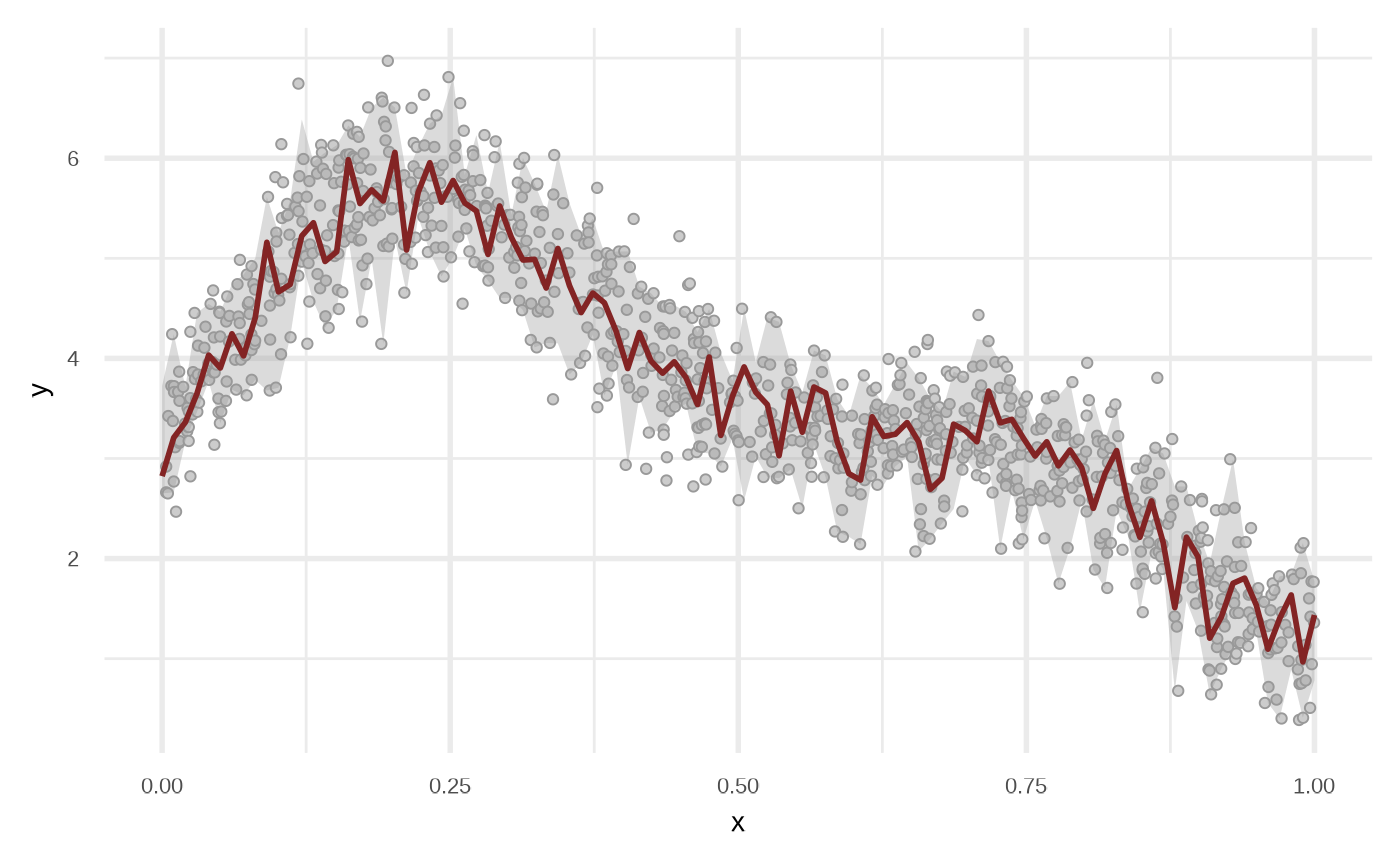
# this will be relative similar to `fit_regression_tree` due
# we are using 1 tree
plot(fit_regression_random_forest(df, ntree = 1, maxdepth = 3))