Quasi Anscombe data sets

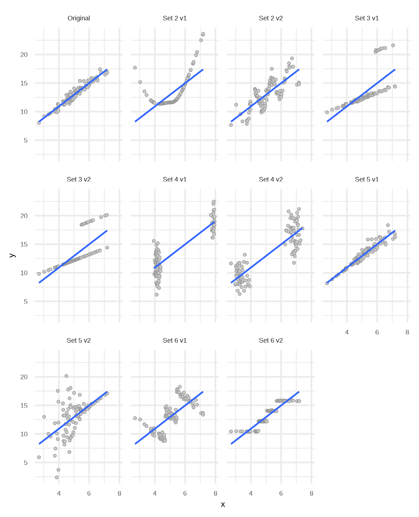
The sets

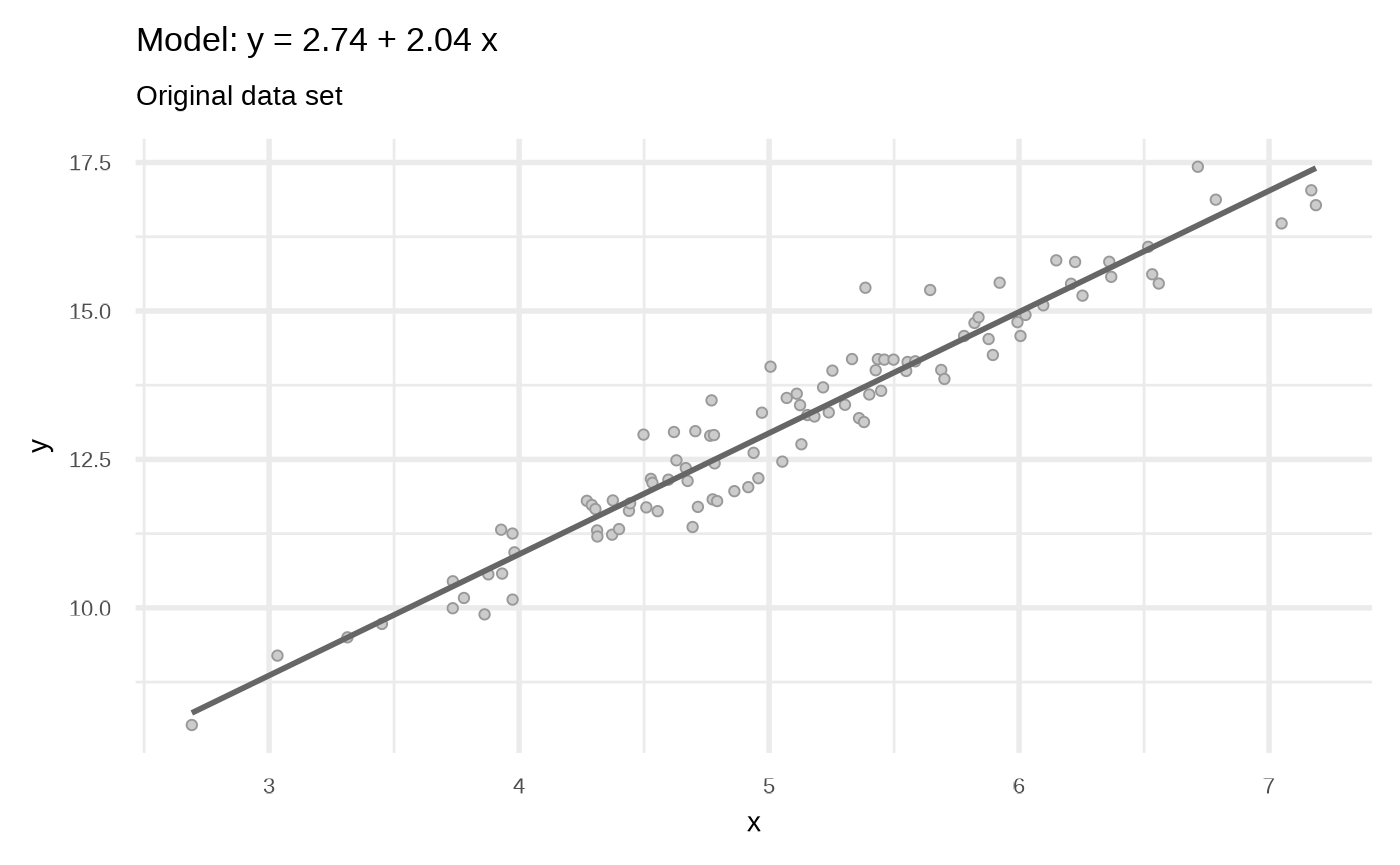
Set 1: The original

library(klassets)
library(ggplot2)

set.seed(123)

df <- sim_quasianscombe_set_1(n = 100, beta1 = 2)

plot(df) +
  # xlim(0, NA) +
  # ylim(0, NA) +
  labs(subtitle = "Original data set")

Set 4: No linear relationship

func <- function(x) 1.5 * x^2

df2_1 <- sim_quasianscombe_set_2(df, residual_factor = 0, fun = func)

funktion <- function(x){ 2 * sin(x*diff(range(x))) }

df2_2 <- sim_quasianscombe_set_2(df, fun = funktion, residual_factor = 1.25)

Set 3: Extreme values

df3_1 <- sim_quasianscombe_set_3(df, prop = 0.10)

df3_2 <- sim_quasianscombe_set_3(df, prop = 0.15, residual_factor = 0)

Set 4: Clusters

df4_1 <- sim_quasianscombe_set_4(df, prop = 0.25)

df4_2 <- sim_quasianscombe_set_4(df, rescale_to = c(0, .1), prop = 0.5)

Set 5: Heteroskedasticity

df5_1 <- sim_quasianscombe_set_5(df, residual_factor = 2)

df5_2 <- sim_quasianscombe_set_5(df, fun = function(x) rev(x**2))

Set 6: Simpson’s Paradox

df6_1 <- sim_quasianscombe_set_6(df, residual_factor = 1)

df6_2 <- sim_quasianscombe_set_6(df, groups = 4, b1_factor = 0, residual_factor = 0.1)

Combine results

library(dplyr, warn.conflicts = FALSE)
library(tidyr)
library(purrr)
library(broom)

dfs <- list(
  "Original" = df,
  "Set 2 v1" = df2_1,
  "Set 2 v2" = df2_2,
  "Set 3 v1" = df3_1,
  "Set 3 v2" = df3_2,
  "Set 4 v1" = df4_1,
  "Set 4 v2" = df4_2,
  "Set 5 v1" = df5_1,
  "Set 5 v2" = df5_2,
  "Set 6 v1" = df6_1,
  "Set 6 v2" = df6_2
)

dfs <- dfs |> 
  tibble::enframe(name = "set") |> 
  tidyr::unnest(cols = c(value))

From [@warnes](https://github.com/warnes) gtools package

stars.pval <- function(p.value) {
  unclass(
    symnum(p.value,
      corr = FALSE, na = FALSE,
      cutpoints = c(0, 0.001, 0.01, 0.05, 0.1, 1),
      symbols = c("***", "**", "*", ".", " ")
    )
  )
}

Visual representation of the data sets

pxy <- ggplot(dfs, aes(x, y)) +
  geom_point(shape = 21, fill = "gray80", color = "gray60") +
  geom_smooth(method = "lm", se = FALSE, formula = y ~ x) +
  facet_wrap(vars(set))

pxy

Checking Coefficients and its significance

df_mods <- dfs |> 
  dplyr::group_nest(set) |> 
  dplyr::mutate(
    model = map(data, lm, formula = y ~ x),
    parameters = map(model, broom::tidy)
    # value = map(model, coefficients),
    # coef  = map(value, names)
    ) 

dfcoef <- df_mods |> 
  dplyr::select(set, parameters) |> 
  tidyr::unnest(cols = c(parameters)) |> 
  dplyr::mutate(sig = stars.pval(p.value))

dfcoef
#> # A tibble: 22 × 7
#>    set      term        estimate std.error statistic  p.value sig  
#>    <chr>    <chr>          <dbl>     <dbl>     <dbl>    <dbl> <chr>
#>  1 Original (Intercept)     2.74    0.276       9.93 1.74e-16 ***  
#>  2 Original x               2.04    0.0533     38.3  1.01e-60 ***  
#>  3 Set 2 v1 (Intercept)     2.74    1.18        2.33 2.20e- 2 *    
#>  4 Set 2 v1 x               2.04    0.228       8.97 2.11e-14 ***  
#>  5 Set 2 v2 (Intercept)     2.74    0.898       3.05 2.94e- 3 **   
#>  6 Set 2 v2 x               2.04    0.174      11.8  1.95e-20 ***  
#>  7 Set 3 v1 (Intercept)     2.74    1.15        2.37 1.97e- 2 *    
#>  8 Set 3 v1 x               2.04    0.223       9.14 8.86e-15 ***  
#>  9 Set 3 v2 (Intercept)     2.74    1.05        2.61 1.06e- 2 *    
#> 10 Set 3 v2 x               2.04    0.203      10.0  9.74e-17 ***  
#> # … with 12 more rows

dfcoef |> 
  dplyr::select(set, term, estimate) |> 
  tidyr::pivot_wider(names_from = "term", values_from = "estimate")
#> # A tibble: 11 × 3
#>    set      `(Intercept)`     x
#>    <chr>            <dbl> <dbl>
#>  1 Original          2.74  2.04
#>  2 Set 2 v1          2.74  2.04
#>  3 Set 2 v2          2.74  2.04
#>  4 Set 3 v1          2.74  2.04
#>  5 Set 3 v2          2.74  2.04
#>  6 Set 4 v1          2.74  2.04
#>  7 Set 4 v2          2.74  2.04
#>  8 Set 5 v1          2.74  2.04
#>  9 Set 5 v2          2.74  2.04
#> 10 Set 6 v1          2.74  2.04
#> 11 Set 6 v2          2.74  2.04