Binary classification
Source:vignettes/articles/Binary-classification.Rmd
Binary-classification.RmdGenerating data set
The main function is sim_response_xy, you need to
define:
- A number of observations to simulate.
- Distributions to sample
and
.
For example
purrr::partial(runif, min = -1, max = 1). - A function to define the relation between the response and the
and
,
for example
function(x, y) x > yThis function must return a logical value. - A number to define the noise in the generated data.
library(klassets)
library(ggplot2)
library(patchwork)

set.seed(123)

df_default <- sim_response_xy(n = 500)

df_default
#> # A tibble: 500 × 3
#>    response       x        y
#>    <fct>      <dbl>    <dbl>
#>  1 FALSE    -0.425  -0.293
#>  2 TRUE      0.577  -0.267
#>  3 FALSE    -0.182  -0.426
#>  4 TRUE      0.766  -0.840
#>  5 TRUE      0.881  -0.269
#>  6 FALSE    -0.909  -0.644
#>  7 FALSE     0.0562  0.0721
#>  8 TRUE      0.785   0.00790
#>  9 TRUE      0.103   0.890
#> 10 TRUE     -0.0868 -0.317
#> # ℹ 490 more rows

plot(df_default)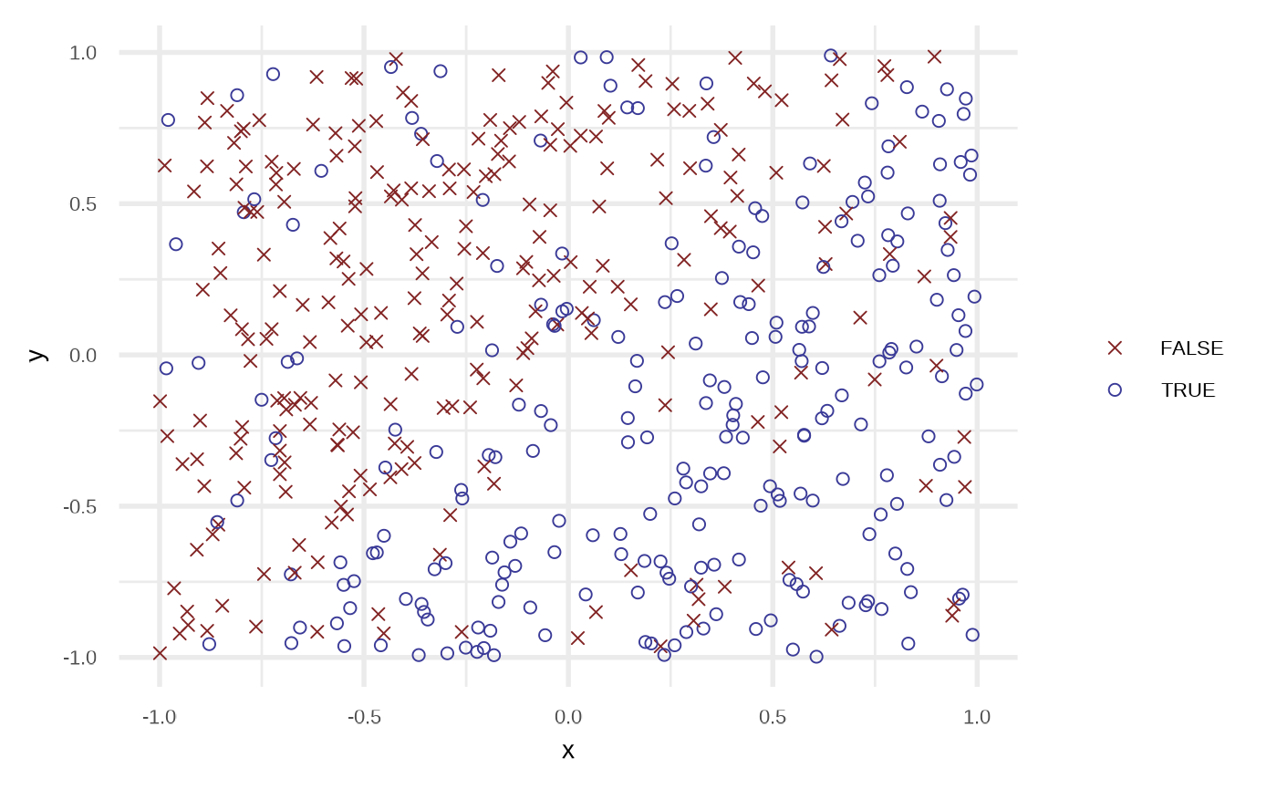
df <- sim_response_xy(
  n = 500,
  x_dist = purrr::partial(runif, min = -1, max = 1),
  # relationship = function(x, y) sqrt(abs(x)) - x - 0.5 > sin(y),
  relationship = function(x, y) sin(x*pi) > sin(y*pi),
  noise = 0.15
  )

plot(df)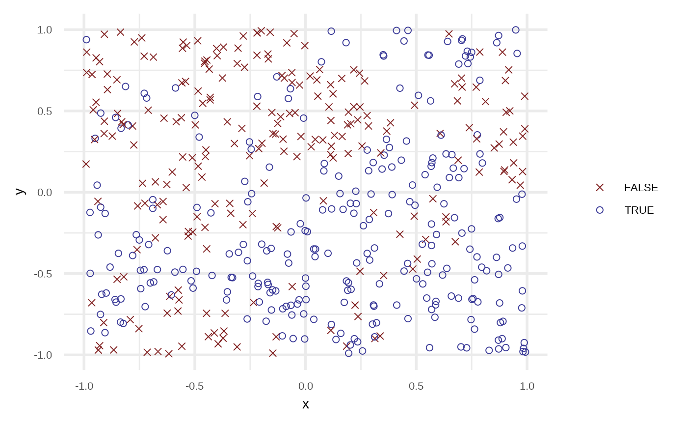
Fit classification algorithms
Logistic Regression
df_lr <- fit_logistic_regression(df)

df_lr
#> # A tibble: 500 × 4
#>    response       x       y prediction
#>    <fct>      <dbl>   <dbl>      <dbl>
#>  1 TRUE      0.876  -0.681       0.885
#>  2 TRUE      0.976  -0.711       0.899
#>  3 TRUE     -0.0874 -0.702       0.745
#>  4 FALSE    -0.539   0.0289      0.385
#>  5 TRUE      0.391  -0.0143      0.637
#>  6 FALSE     0.113   0.233       0.478
#>  7 TRUE      0.169  -0.105       0.614
#>  8 FALSE    -0.133  -0.889       0.785
#>  9 FALSE    -0.148  -0.989       0.807
#> 10 TRUE      0.194  -0.556       0.760
#> # ℹ 490 more rows

plot(df_lr)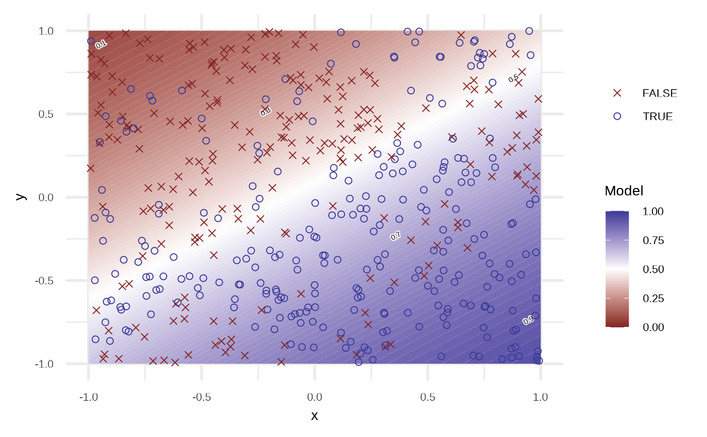
By default the model use order = 1 of the variables,
i.e, response ~ x + y. We can get a better fit if we
increase the order.
df_lr2 <- fit_logistic_regression(df, order = 4, stepwise = TRUE)

attr(df_lr2, "model")
#>
#> Call:  glm(formula = response ~ x + y + x_3 + y_3, family = binomial,
#>     data = df)
#>
#> Coefficients:
#> (Intercept)            x            y          x_3          y_3
#>      0.1533       3.3121      -4.4480      -3.3786       4.6436
#>
#> Degrees of Freedom: 499 Total (i.e. Null);  495 Residual
#> Null Deviance:       690.8
#> Residual Deviance: 518   AIC: 528

plot(df_lr2)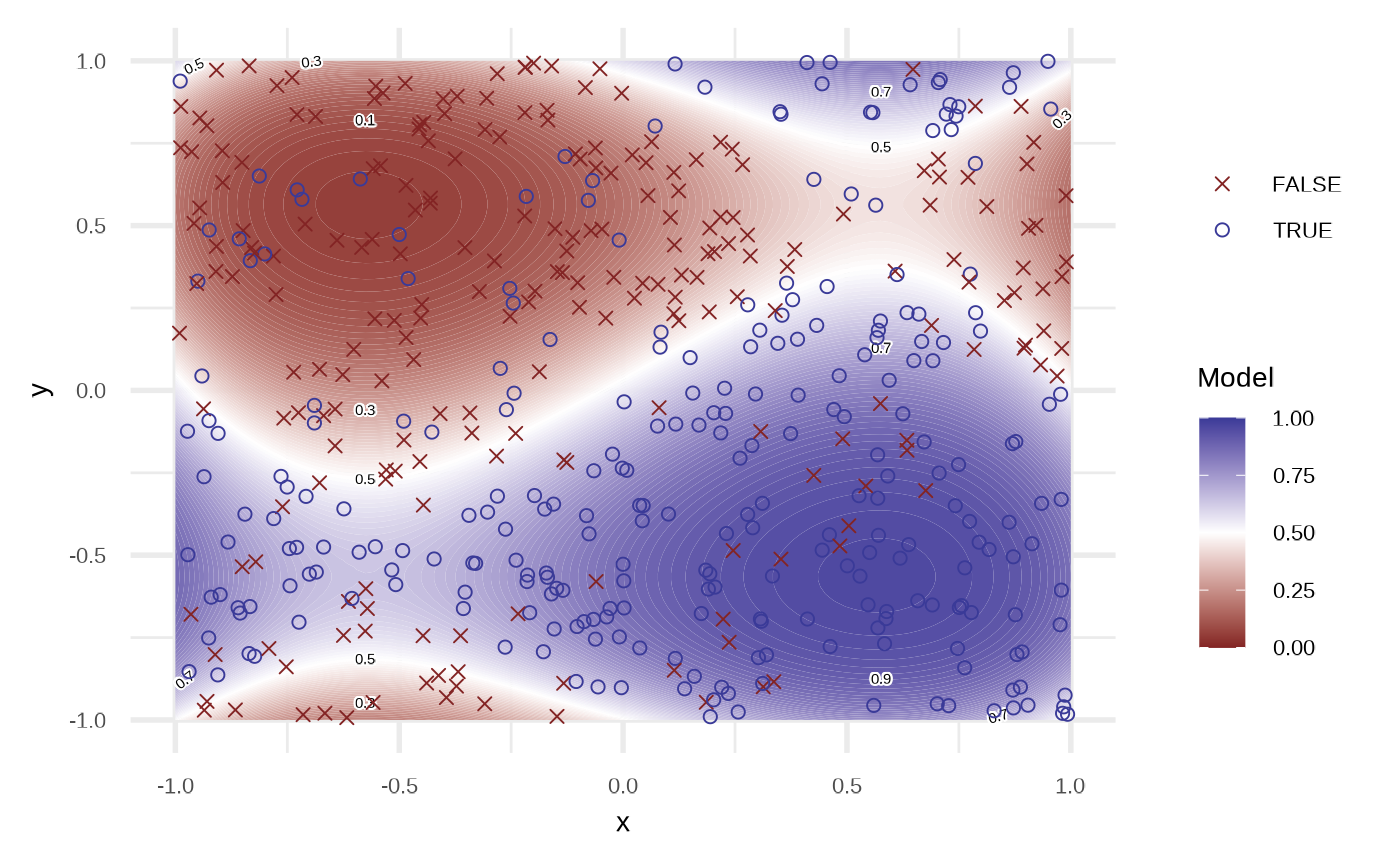
Testing various orders.
orders <- c(1, 2, 3, 4)

orders |>
  purrr::map(fit_logistic_regression, df = df) |>
  purrr::map(plot) |>
  purrr::reduce(`+`) +
  patchwork::plot_layout(guides = "collect") &
  theme_void() + theme(legend.position = "none")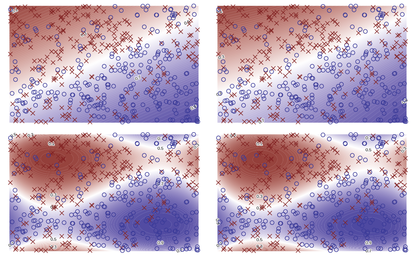
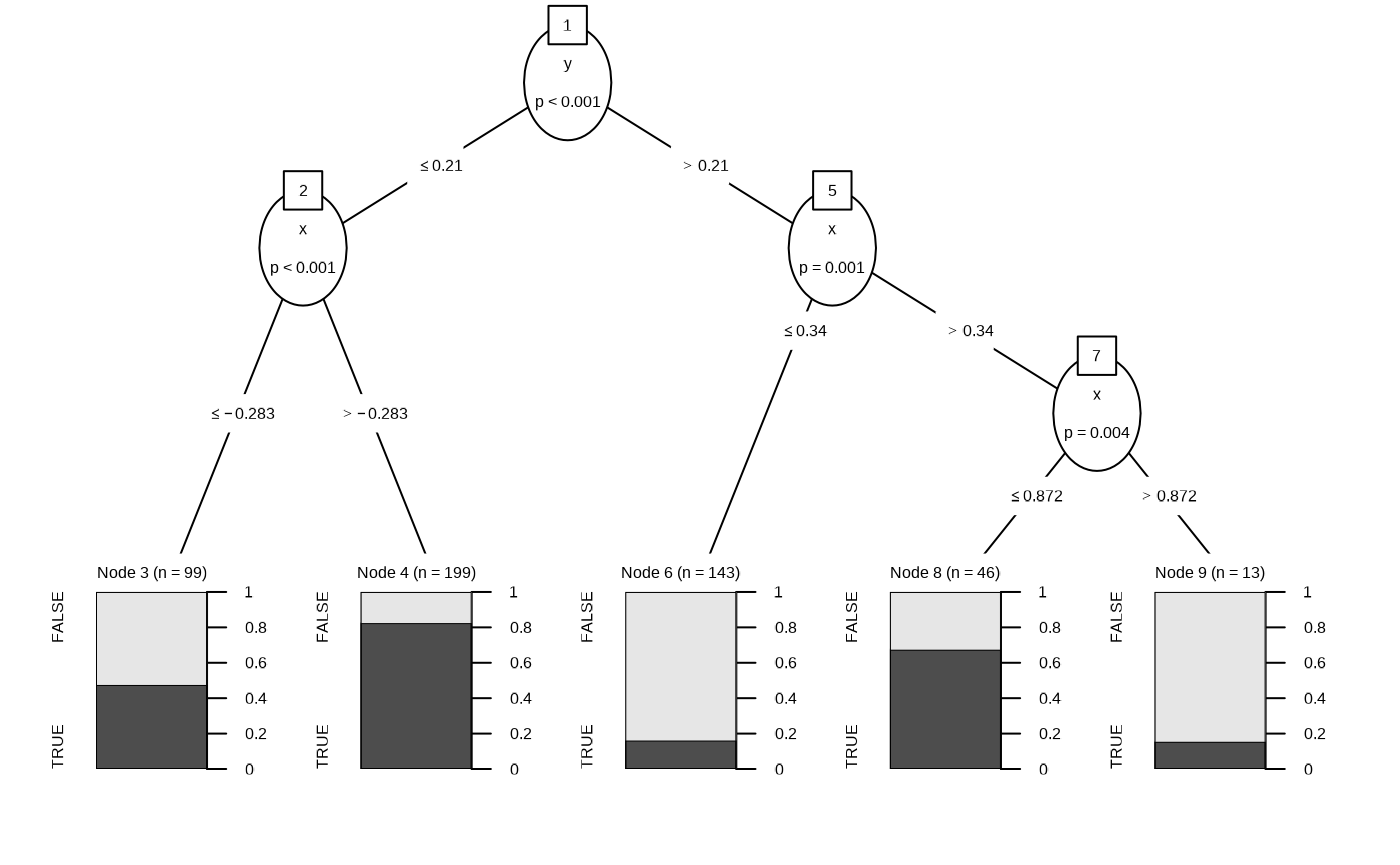
Classification Tree
df_rt <- fit_classification_tree(df)

plot(df_rt)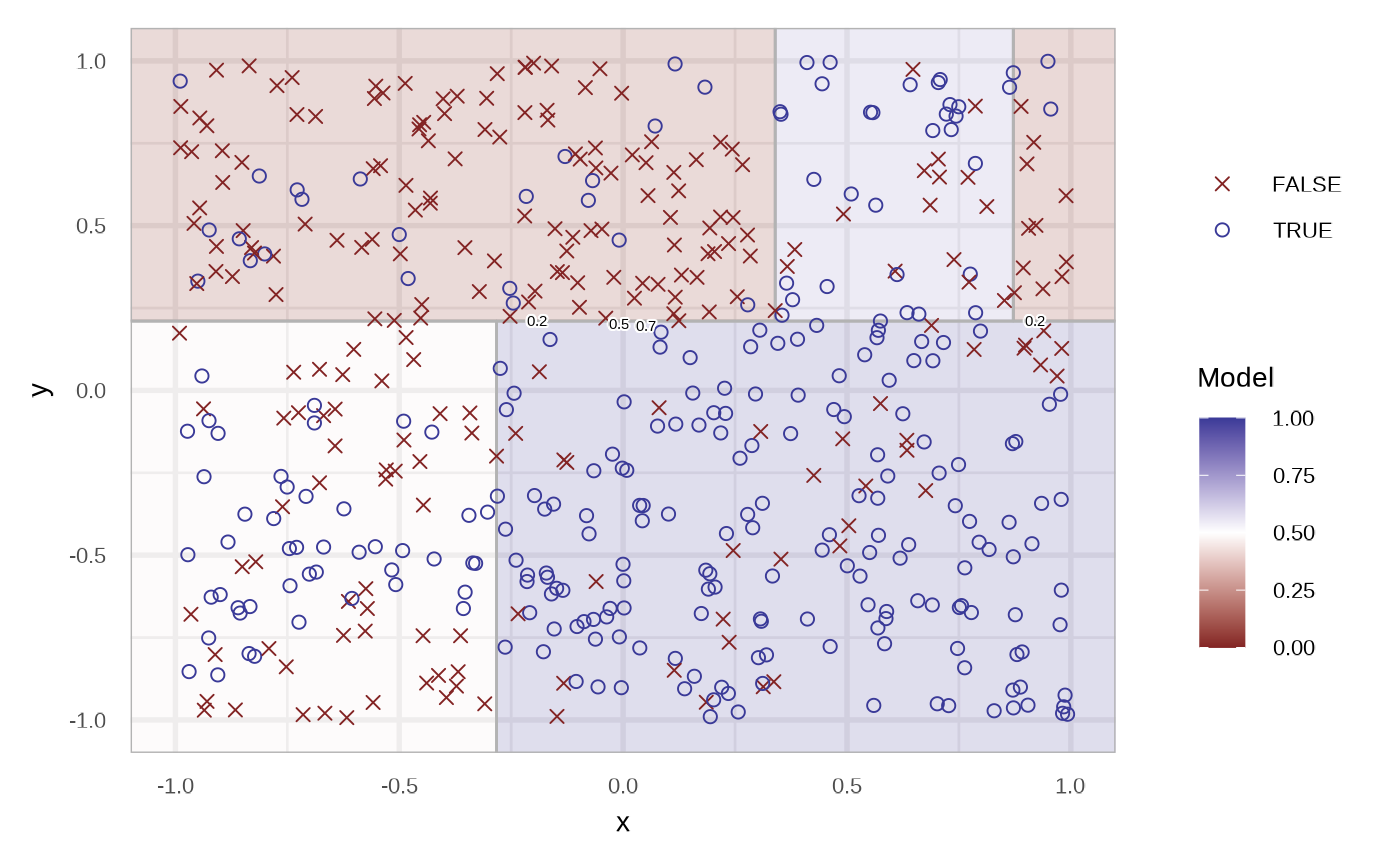
plot(fit_classification_tree(df, alpha = 0.25))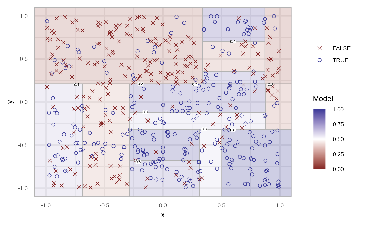
The region are filled with the probability of the respective node. We
can specify the type of the prediction using the type
argument. In the case of response.
df_rt_response <- fit_classification_tree(df, type = "response")

df_rt_response
#> # A tibble: 500 × 4
#>    response       x       y prediction
#>    <fct>      <dbl>   <dbl> <fct>
#>  1 TRUE      0.876  -0.681  TRUE
#>  2 TRUE      0.976  -0.711  TRUE
#>  3 TRUE     -0.0874 -0.702  TRUE
#>  4 FALSE    -0.539   0.0289 FALSE
#>  5 TRUE      0.391  -0.0143 TRUE
#>  6 FALSE     0.113   0.233  FALSE
#>  7 TRUE      0.169  -0.105  TRUE
#>  8 FALSE    -0.133  -0.889  TRUE
#>  9 FALSE    -0.148  -0.989  TRUE
#> 10 TRUE      0.194  -0.556  TRUE
#> # ℹ 490 more rows

plot(df_rt_response)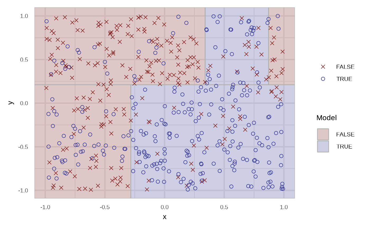
And now for the node.
df_rt_node <- fit_classification_tree(df, type = "node", maxdepth = 3)

df_rt_node
#> # A tibble: 500 × 4
#>    response       x       y prediction
#>    <fct>      <dbl>   <dbl>      <int>
#>  1 TRUE      0.876  -0.681           4
#>  2 TRUE      0.976  -0.711           4
#>  3 TRUE     -0.0874 -0.702           4
#>  4 FALSE    -0.539   0.0289          3
#>  5 TRUE      0.391  -0.0143          4
#>  6 FALSE     0.113   0.233           6
#>  7 TRUE      0.169  -0.105           4
#>  8 FALSE    -0.133  -0.889           4
#>  9 FALSE    -0.148  -0.989           4
#> 10 TRUE      0.194  -0.556           4
#> # ℹ 490 more rows

plot(df_rt_node)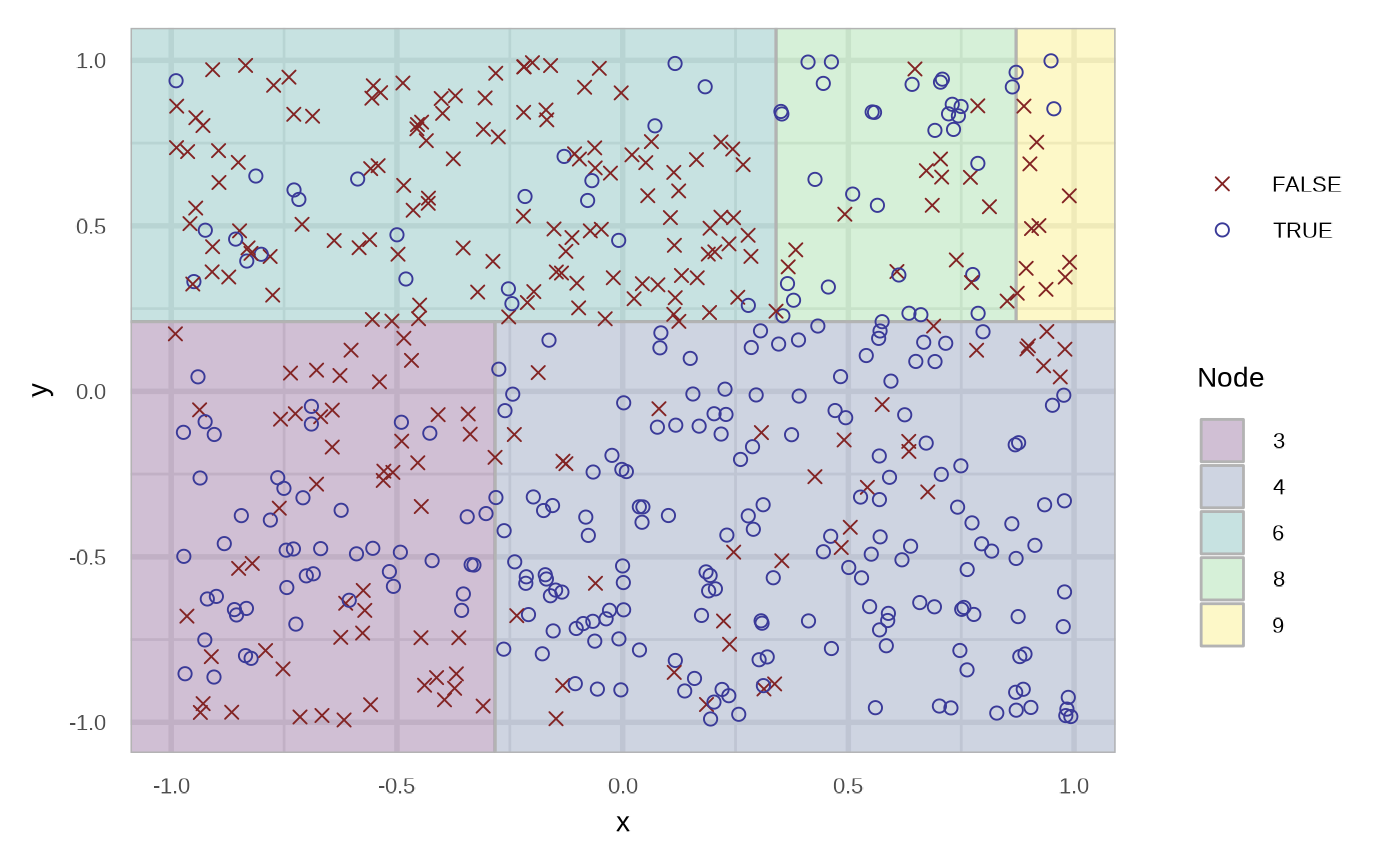
K Nearest Neighbours
With the class::knn implementation.
# defaults to prob
fit_knn(df)
#> # A tibble: 500 × 4
#>    response       x       y prediction
#>    <fct>      <dbl>   <dbl>      <dbl>
#>  1 TRUE      0.876  -0.681         1
#>  2 TRUE      0.976  -0.711         1
#>  3 TRUE     -0.0874 -0.702         1
#>  4 FALSE    -0.539   0.0289        0.9
#>  5 TRUE      0.391  -0.0143        0.8
#>  6 FALSE     0.113   0.233         0.8
#>  7 TRUE      0.169  -0.105         0.9
#>  8 FALSE    -0.133  -0.889         0.8
#>  9 FALSE    -0.148  -0.989         0.6
#> 10 TRUE      0.194  -0.556         0.7
#> # ℹ 490 more rows

fit_knn(df, type = "response")
#> # A tibble: 500 × 4
#>    response       x       y prediction
#>    <fct>      <dbl>   <dbl> <fct>
#>  1 TRUE      0.876  -0.681  TRUE
#>  2 TRUE      0.976  -0.711  TRUE
#>  3 TRUE     -0.0874 -0.702  TRUE
#>  4 FALSE    -0.539   0.0289 FALSE
#>  5 TRUE      0.391  -0.0143 TRUE
#>  6 FALSE     0.113   0.233  FALSE
#>  7 TRUE      0.169  -0.105  TRUE
#>  8 FALSE    -0.133  -0.889  TRUE
#>  9 FALSE    -0.148  -0.989  TRUE
#> 10 TRUE      0.194  -0.556  TRUE
#> # ℹ 490 more rows

plot(fit_knn(df))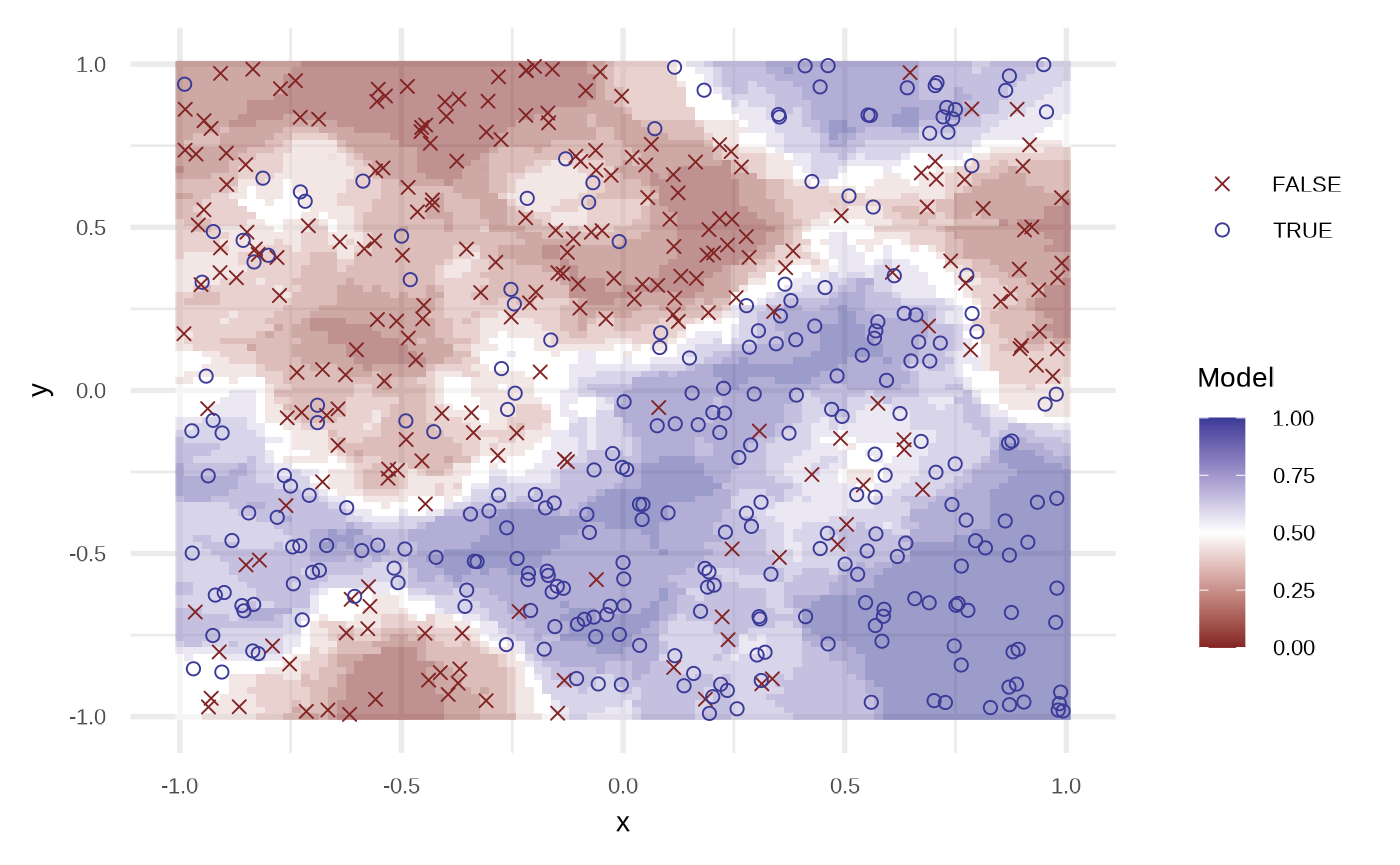
neighbours <- c(3, 10, 50, 300)

purrr::map(neighbours, fit_knn, df = df) |>
  purrr::map(plot) |>
  purrr::reduce(`+`) +
  patchwork::plot_layout(guides = "collect") &
  theme_void() + theme(legend.position = "none")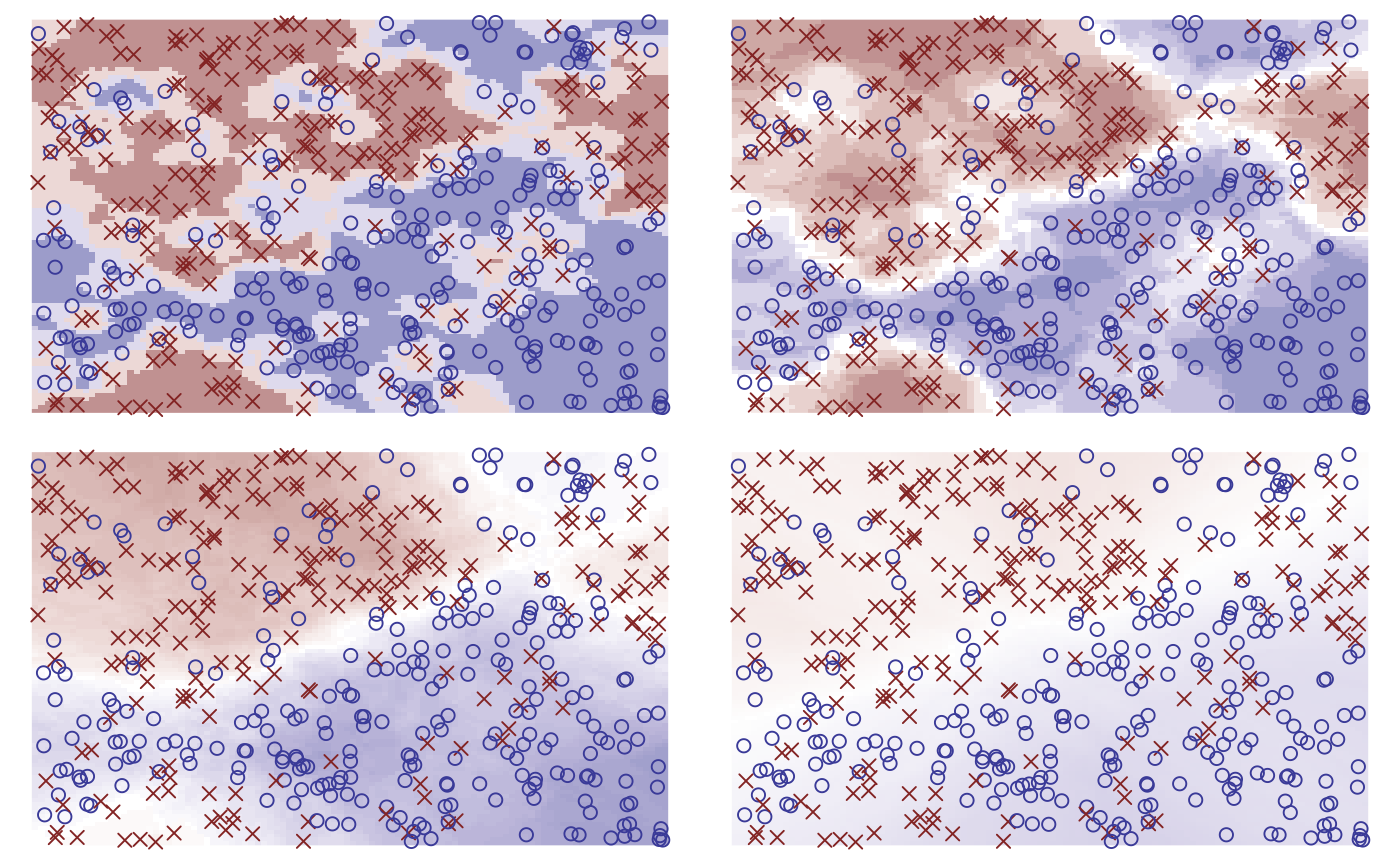
purrr::map(neighbours, fit_knn, df = df, type = "response") |>
  purrr::map(plot) |>
  purrr::reduce(`+`) +
  patchwork::plot_layout(guides = "collect")  &
  theme_void() + theme(legend.position = "none")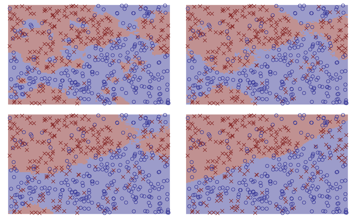
Random Forest
Using the ranger::ranger function.
df_crf <- fit_classification_random_forest(df)

plot(df_crf)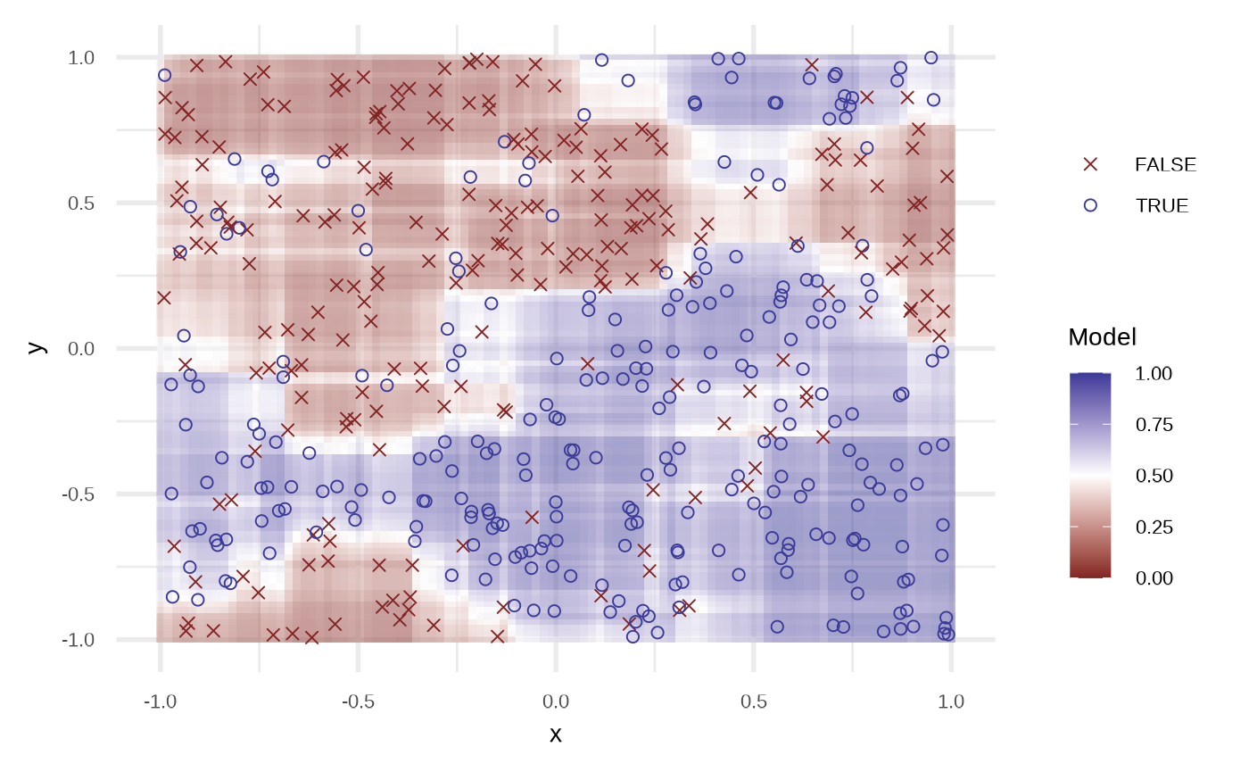
df_crf
#> # A tibble: 500 × 4
#>    response       x       y prediction
#>    <fct>      <dbl>   <dbl>      <dbl>
#>  1 TRUE      0.876  -0.681       0.984
#>  2 TRUE      0.976  -0.711       0.952
#>  3 TRUE     -0.0874 -0.702       0.905
#>  4 FALSE    -0.539   0.0289      0.173
#>  5 TRUE      0.391  -0.0143      0.899
#>  6 FALSE     0.113   0.233       0.264
#>  7 TRUE      0.169  -0.105       0.946
#>  8 FALSE    -0.133  -0.889       0.702
#>  9 FALSE    -0.148  -0.989       0.500
#> 10 TRUE      0.194  -0.556       0.922
#> # ℹ 490 more rows