Generate quasi Anscombe data sets Type 1

This function generate a data set Type 1 creating first a x a random vector then apply a linear transformation using beta0 and beta1 and finally adding a normal distributed noise using error_sd creating y values.

Usage

sim_quasianscombe_set_1(
  n = 500,
  beta0 = 3,
  beta1 = 0.5,
  x_dist = purrr::partial(rnorm, mean = 5, sd = 1),
  error_dist = purrr::partial(rnorm, sd = 0.5)
)

Arguments

n

Number of observations

beta0

beta0, default value: 3,

beta1

beta1, default value: 0.5

x_dist

A random number generation function. Default is a rnorm with mean 5 and sd 1.

error_dist

A random number generation function. Default is a rnorm with mean 0 and sd 0.5.

Details

This is the typical first example when regression analysis is taught.

Internally this is the same procedure of sim_xy.

Examples

df <- sim_quasianscombe_set_1()

df
#> # A tibble: 500 × 2
#>        x     y
#>    <dbl> <dbl>
#>  1  2.22  3.65
#>  2  2.29  4.97
#>  3  2.60  3.40
#>  4  2.76  4.51
#>  5  2.83  3.95
#>  6  3.05  3.83
#>  7  3.07  5.01
#>  8  3.07  4.90
#>  9  3.14  4.61
#> 10  3.15  4.76
#> # … with 490 more rows

plot(df)


plot(df, add_lm = FALSE)


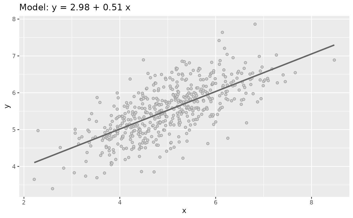
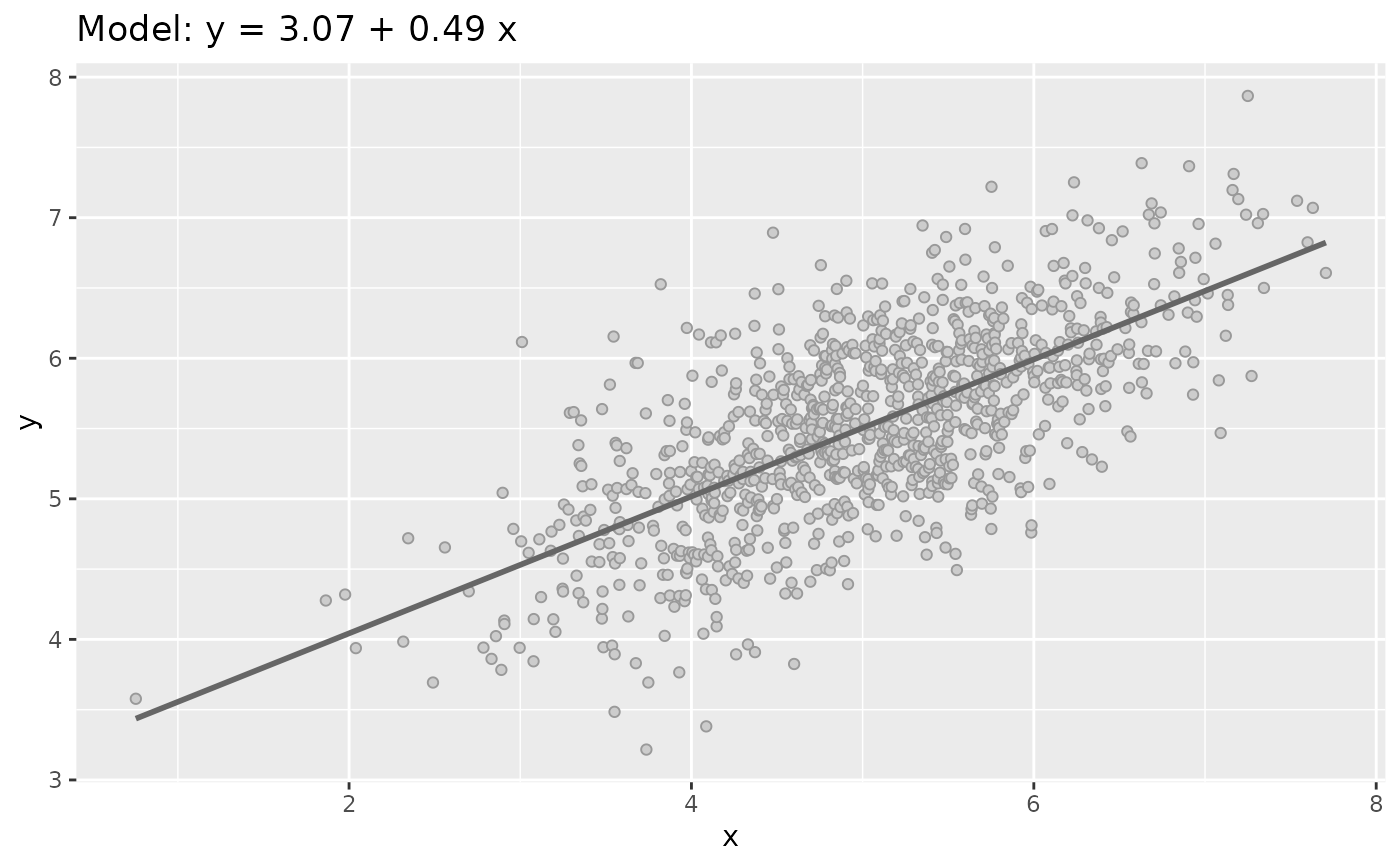
plot(sim_quasianscombe_set_1(n = 1000))


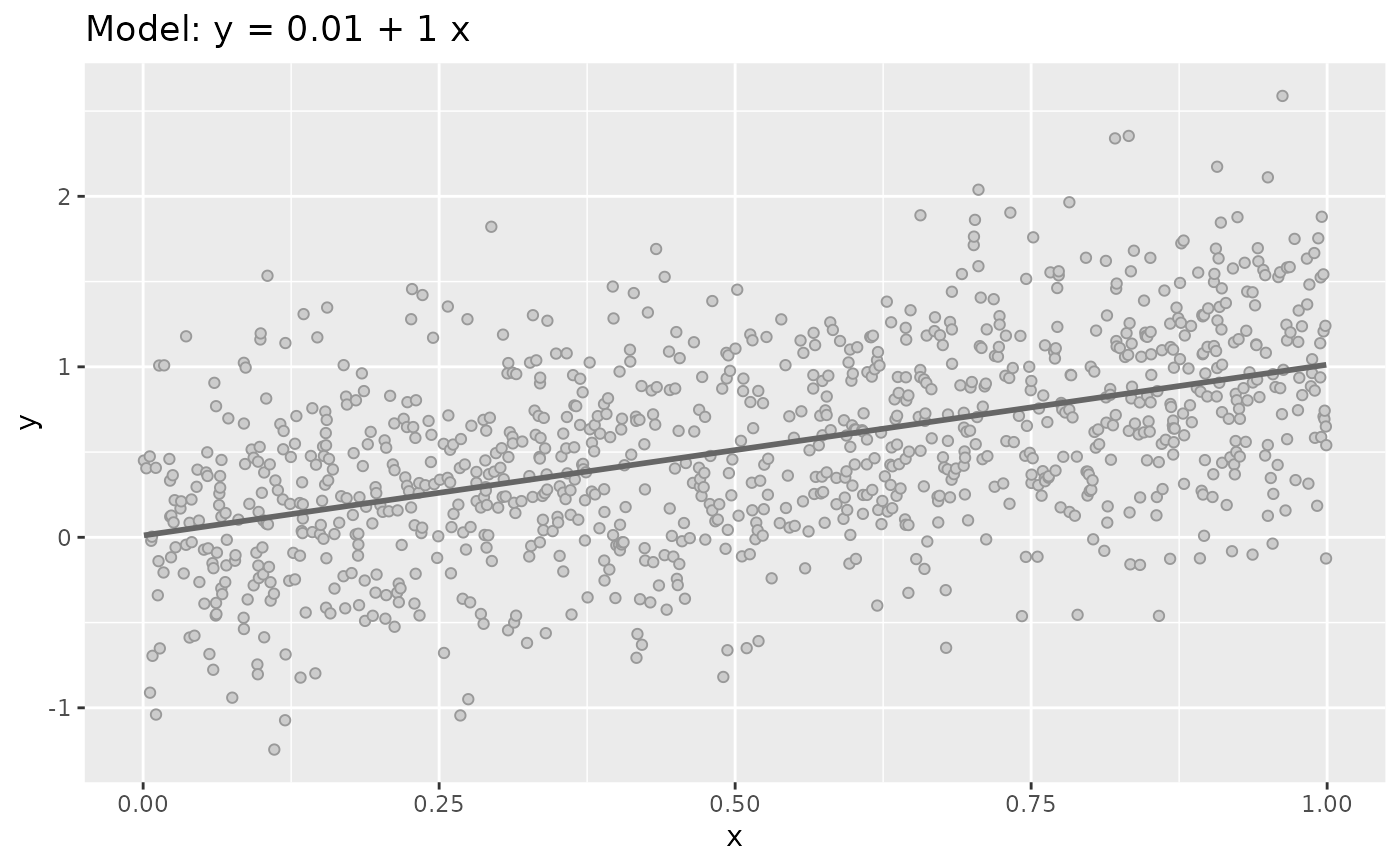
plot(sim_quasianscombe_set_1(n = 1000, beta0 = 0, beta1 = 1, x_dist = runif))