Generate quasi Anscombe data sets Type 2: No linear relationship

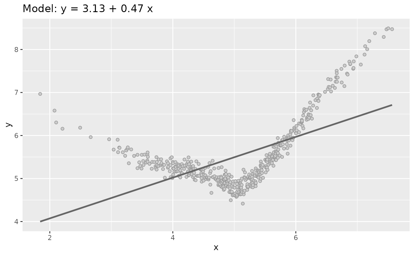
Data sets Type 2 shows how a no linear realtionship between x and y can lead in the same regression model (in terms of parameter values) of the Type 1.

Usage

sim_quasianscombe_set_2(
  df,
  fun = function(x) {
     x^2
 },
  residual_factor = 0.25
)

Arguments

df

A data frame from sim_quasianscombe_set_1 (or similar).

fun

A function to apply, this is applied to normalized version of x.

residual_factor

Numeric value to multiply residual to modify their variance.

Examples

df <- sim_quasianscombe_set_1()

dataset2 <- sim_quasianscombe_set_2(df)

dataset2
#> # A tibble: 500 × 2
#>        x     y
#>    <dbl> <dbl>
#>  1  1.84 14.1 
#>  2  2.08 12.4 
#>  3  2.10 12.0 
#>  4  2.21 11.3 
#>  5  2.49 10.0 
#>  6  2.67  9.09
#>  7  2.96  7.95
#>  8  3.04  7.47
#>  9  3.10  7.50
#> 10  3.11  7.19
#> # … with 490 more rows

plot(dataset2)


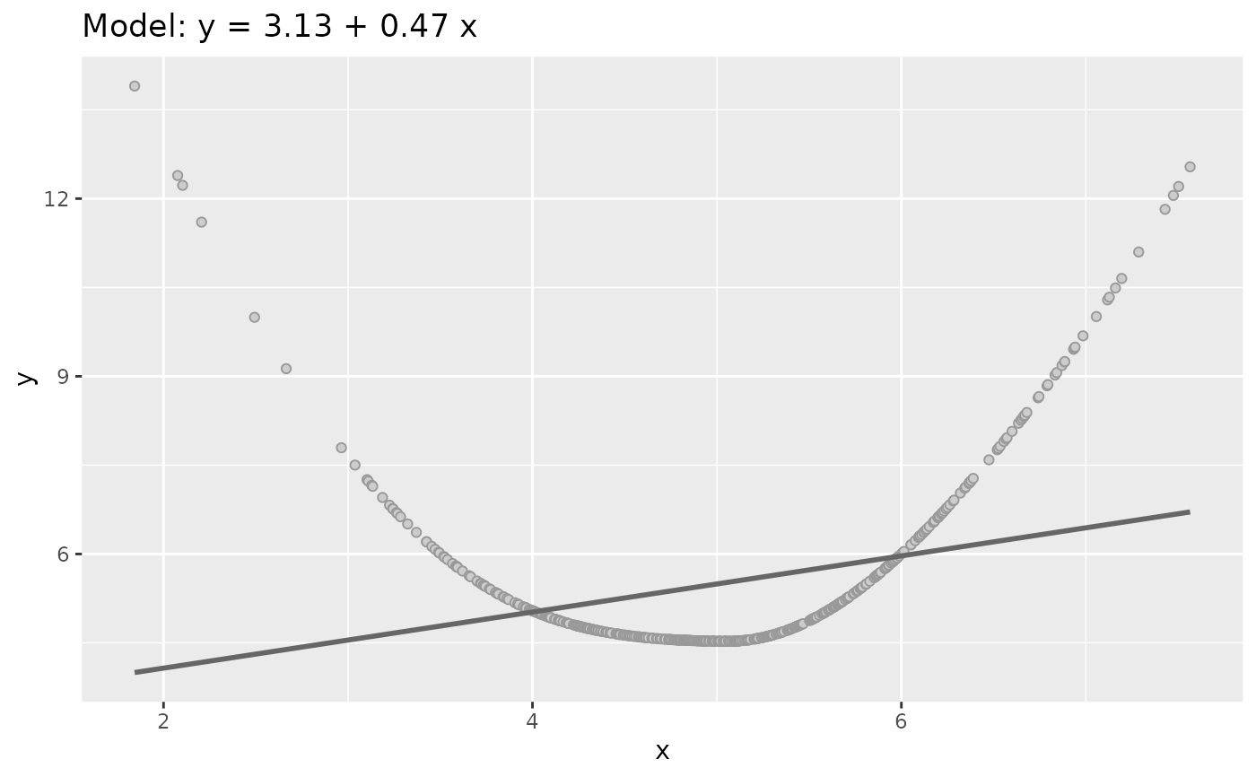
plot(sim_quasianscombe_set_2(df, residual_factor = 0))


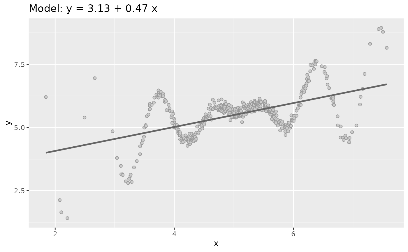
fun1 <- function(x){ 2 * sin(x*diff(range(x))) }

plot(sim_quasianscombe_set_2(df, fun = fun1))


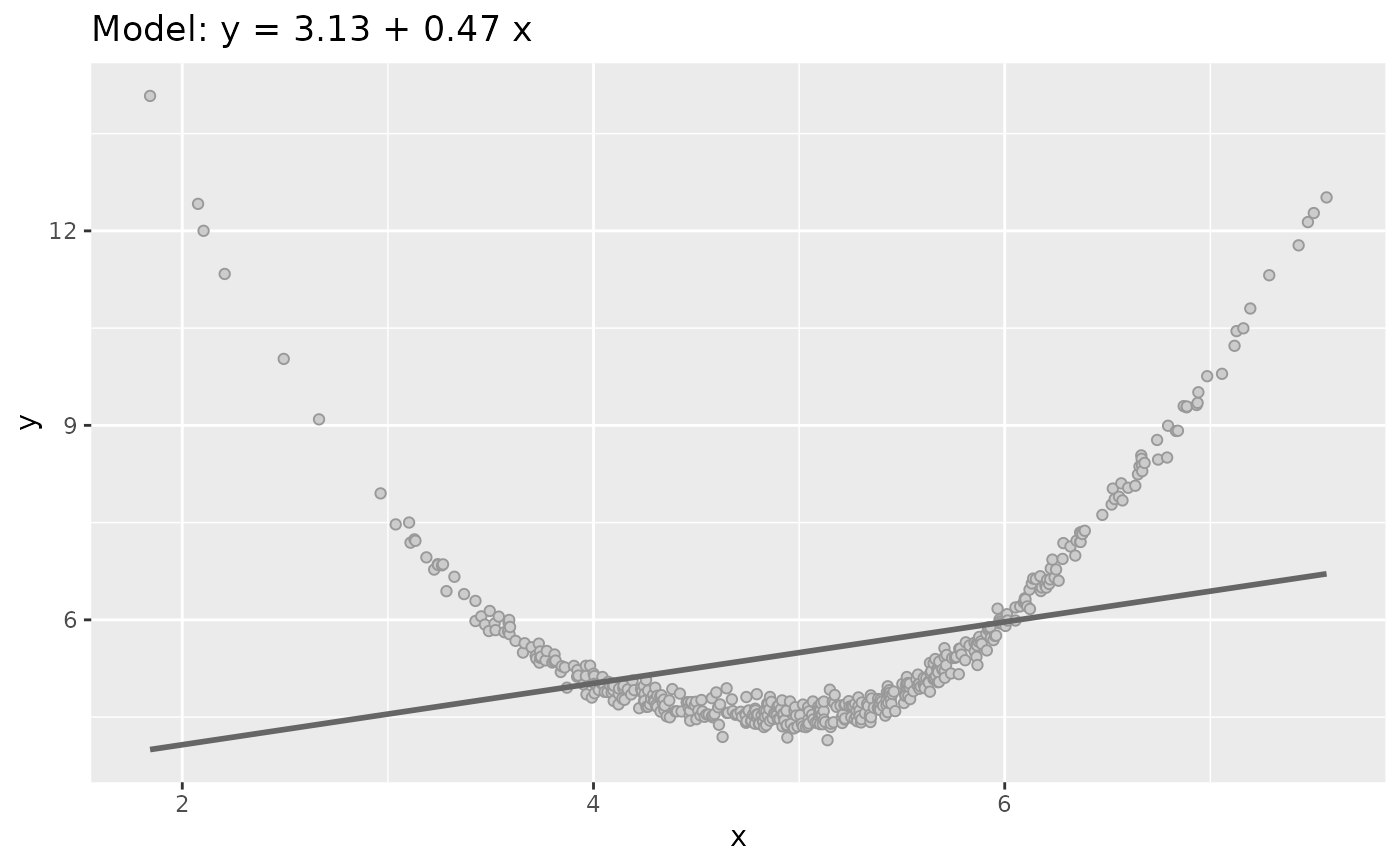
fun2 <- abs

plot(sim_quasianscombe_set_2(df, fun = fun2))


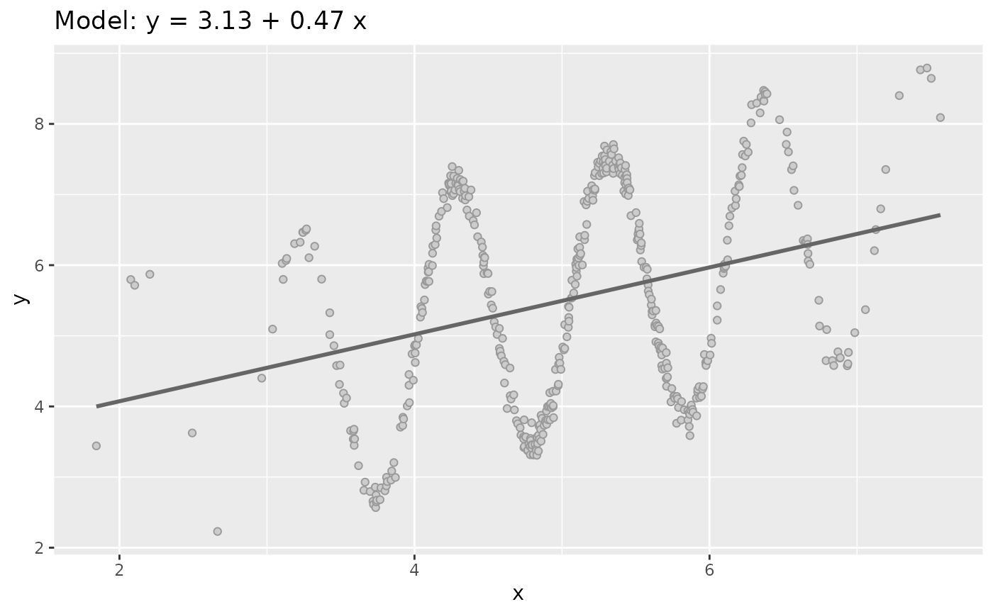
fun3 <- function(x){ (x - mean(x)) * sin(x*diff(range(x))) }

plot(sim_quasianscombe_set_2(df, fun = fun3))