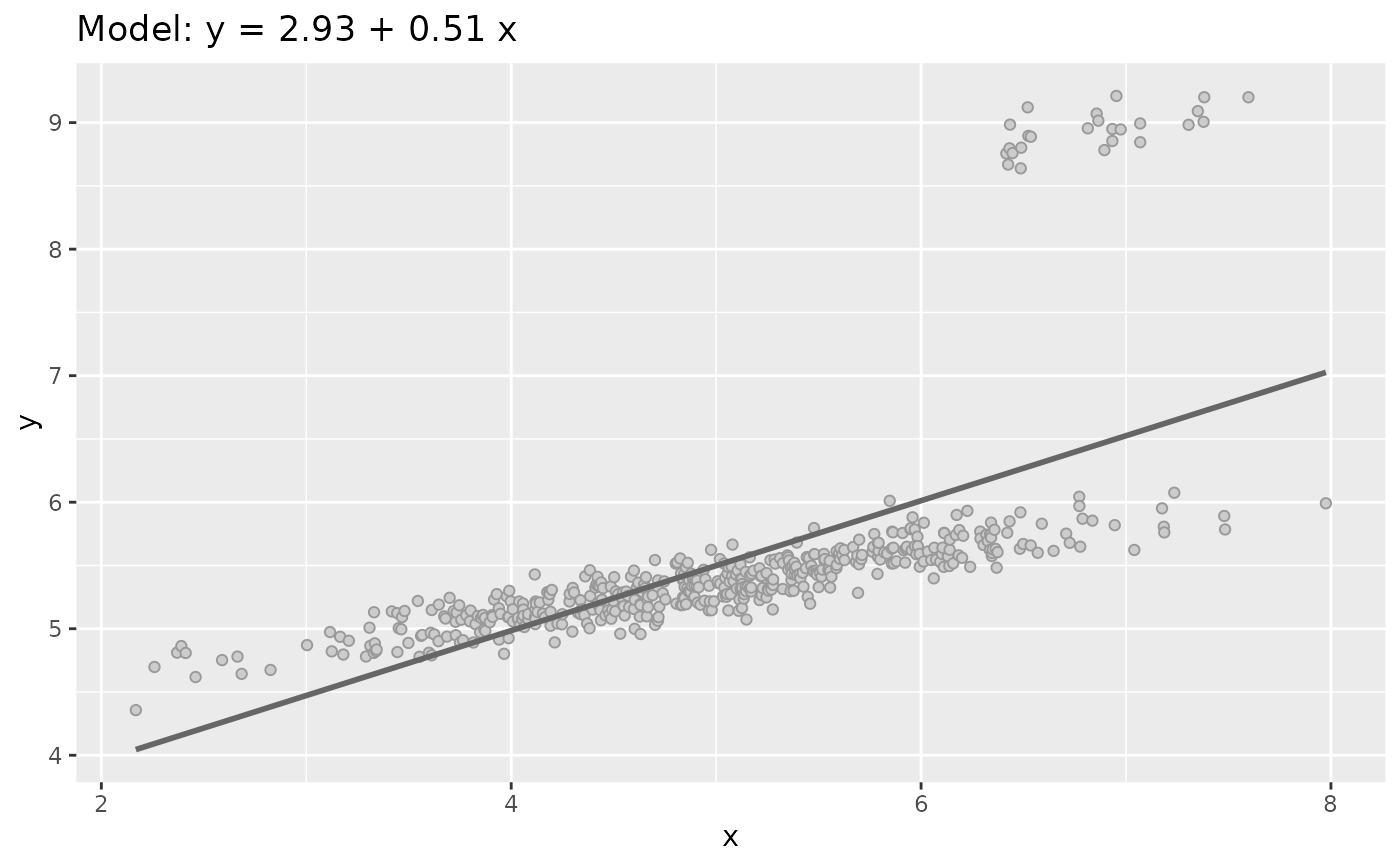
Generate quasi Anscombe data sets Type 3: Extreme values (a.k.a Outliers)
Source:R/quasianscombe.R
sim_quasianscombe_set_3.RdData sets Type 3 get some outliers but conserving the $x$ mean and the same coefficients -but different significance- of the adjusted linear model.
Details
This function will:
Calculate the linear regression model and will calculate new trend using 0.5 times beta1
Take
prop% values from the greater2*propxvalues and modify the relatedyvalue to get the original estimation ofbeta1Apply
residual_factorfactor to residual to get minor variance and better visual impression of the outliers effect.
Examples
df <- sim_quasianscombe_set_1()

dataset3 <- sim_quasianscombe_set_3(df)

dataset3
#> # A tibble: 500 × 2
#>        x     y
#>    <dbl> <dbl>
#>  1  2.17  4.36
#>  2  2.26  4.70
#>  3  2.37  4.81
#>  4  2.39  4.86
#>  5  2.41  4.81
#>  6  2.46  4.62
#>  7  2.59  4.75
#>  8  2.66  4.78
#>  9  2.68  4.64
#> 10  2.83  4.67
#> # ℹ 490 more rows

plot(dataset3)


plot(sim_quasianscombe_set_3(df, prop = 0.1, residual_factor = 0))
