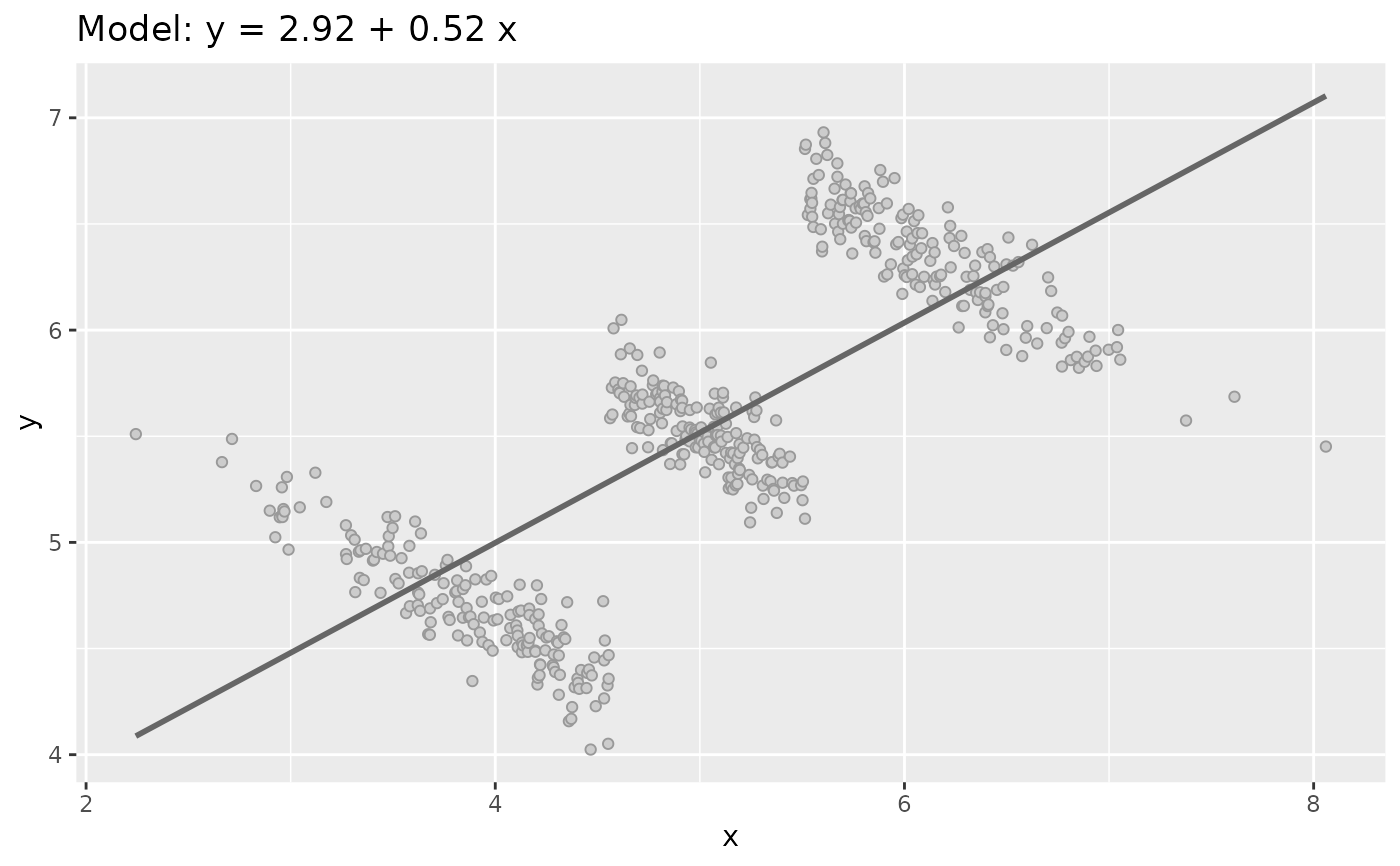
Generate quasi Anscombe data sets Type 6: Simpson's Paradox — sim_quasianscombe_set

Data sets Type 6 recreates the phenomenon of Simpon's paradox.

Usage

sim_quasianscombe_set_6(df, groups = 3, b1_factor = -1, residual_factor = 0.25)

Arguments

df: A data frame from sim_quasianscombe_set_1 (or similar).
groups: Number of groups to separate x values.
b1_factor: A numeric value get the slope in each group from $beta_1$.
residual_factor: Numeric value to multiply residual to modify their variance.

Details

This function will take x vector and separate groups groups to apply a local model with a modified regression using the b1_factor factor.

The residual will be multiply with a value between 0 and 1 to make the visual effect greater.

Examples


df <- sim_quasianscombe_set_1()

dataset6 <- sim_quasianscombe_set_6(df)

dataset6
#> # A tibble: 500 × 2
#>        x     y
#>    <dbl> <dbl>
#>  1  2.24  5.51
#>  2  2.66  5.38
#>  3  2.71  5.49
#>  4  2.83  5.27
#>  5  2.90  5.15
#>  6  2.92  5.02
#>  7  2.95  5.12
#>  8  2.96  5.26
#>  9  2.96  5.13
#> 10  2.96  5.12
#> # … with 490 more rows

plot(dataset6)